• **the observation**, before any math: point a tripod-mounted camera at a static, evenly-lit gray patch and shoot a burst. Each pixel *should* read one constant value; instead it **fluctuates** frame to frame, and across the patch (it should be flat) it's grainy. Two faces of the same thing — noise as **fluctuation over time** and **fluctuation over space when the answer should be constant**. [`fig-averaging-N-frames`]
• **the naive algorithm** is a one-liner: sum the frames, divide by $N$.
```
mean = zeros_like(imSeq[0])
for im in imSeq: mean += im
mean /= len(imSeq)
```
Visibly, 1 → 3 → 5 → 45 frames: the gray patch's histogram tightens, dark areas clean up. *Why* — and *how fast*? [`fig-averaging-N-frames`]
• **the model** (the load-bearing assumption): each pixel's value in frame $i$ is the **true signal plus noise**, $X_i = \mu + n_i$, where the noise is **zero-mean** ($\mathbb{E}[n_i]=0$ — averaging only works if the noise has no DC offset) and **independent** across frames (frame $i$'s noise tells you nothing about frame $j$'s — true for shot & read noise, *false* for fixed-pattern noise; flag this now, fix it in *Calibration*). Each has variance $\operatorname{Var}[n_i]=\sigma^2$.
• **the two tools** (state them as the reusable algebra): for a random variable, scaling squares the variance, $\operatorname{Var}[kX]=k^2\operatorname{Var}[X]$; and for **independent** variables, **variance of the sum is the sum of variances**, $\operatorname{Var}[\sum_i X_i]=\sum_i\operatorname{Var}[X_i]$ (independence is what kills the cross terms / covariance). [`fig-iid-variance-adds`]
• **the derivation** (two lines): the average is $\bar X=\tfrac1N\sum_i X_i$. Its **mean is the true value** — $\mathbb{E}[\bar X]=\tfrac1N\sum_i\mathbb{E}[X_i]=\mu$ — so averaging is **unbiased**: it doesn't distort the signal. Its **variance**: pull out the $\tfrac1N$ (squares, by the first rule), then add (by independence):
$$\operatorname{Var}[\bar X]=\frac{1}{N^2}\operatorname{Var}\Big[\sum_i X_i\Big]=\frac{1}{N^2}\cdot N\sigma^2=\frac{\sigma^2}{N}.$$
Take the square root for the human-readable number: $\sigma_{\bar X}=\sigma/\sqrt N$.
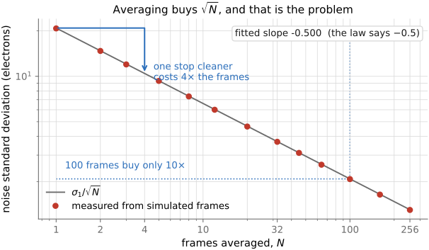
• 💡 **the punchline — the $1/\sqrt N$ law** (see the big-lesson box above): **variance drops as $1/N$, std as $1/\sqrt N$.** This is the chapter's whole quantitative content. Its sting is the diminishing return: $4\times$ the frames for $1\times$ less noise (one stop); 100 frames buys a $10\times$ cleaner image, not 100×. In SNR terms, $+10\log_{10}N$ dB — about **3 dB per doubling**. [`fig-sqrtN-curve`]
• **estimating the noise itself** (aside, for the analysis pipeline): from the same stack you can *measure* $\sigma^2$ per pixel — but divide by $N-1$, not $N$ (**Bessel's correction**), because you used the same samples to estimate the mean, which correlates the residuals and otherwise *under*-estimates the variance. The coin-flip-with-$N{=}2$ example makes this concrete: the $N$ estimator averages to half the true variance; the $N{-}1$ estimator is unbiased.
• **what it confirms about the sensor** (callback to the noise part): map the measured $\sigma$ across a real scene and it tracks the noise sources — more noise (numerically) in **bright** areas (shot noise $\propto\sqrt{\#\text{photons}}$), yet **better SNR** there; the log-SNR image "looks like the photo." Averaging lowers the floor uniformly; it does not change *which* source dominates where.