BookNotesSlidesP-sets Syllabusdraft · v0.2.49.1
💬Comments welcome. To leave a note, select any text and click the note / highlight button that pops up — or open the panel with the tab at the top-right (‹). Notes are visible only inside our private review group.
Computational Photography, an AI-powered Slopendium — 10 Edges matter
expand to📖 Full book outline1 parts · 10 chapters · 58 sections · 8 figures embedded · 4 placeholders · double-click a figure to enlarge
▸Part 10 EDGES MATTER⧉
<!--uid: edges-matter-->
The thread of this part is that **where the edges are** governs the edit. Edges carry most of an image's meaning, so three families of method are organized around them: **gradient-domain (Poisson) editing** reconstructs an image *from* its edges (seamless cloning, gradient-domain HDR, photomontage); **edge-preserving filtering** smooths everything *except* across edges (bilateral, guided, local Laplacian, non-local means → tone mapping, detail, denoising); and **seam optimization** cuts *along* the least-noticeable edges (seam carving, graph-cut compositing). All three lean on the linear-systems and convolution machinery from earlier parts; they belong together because they share one idea — respect the edges.
▸10.1 Bilateral filtering⧉
10.1.7 Anisotropic diffusion and robust estimators⧉
▸10.2 Non-local means⧉
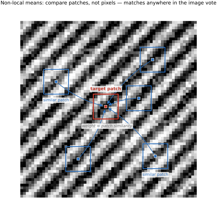
fig-nlmeans-patches
fig-nlmeans-patches · non-local means: compare *patches* not pixels — similar patches elsewhere vote for the center pixel (NL-means) ✅
⬜ figure not yet created
interactive weight-map demo [fig-nlmeans-demo] fig-nlmeans-demo
• chapter intro: split out of [[Non-local means and BM3D]]; NL-means is the bilateral filter living in patch space, and the reason image self-similarity denoises so well.
▸10.3 Edge-preserving optimization — colorization⧉
• **the shift — filtering → optimization**: instead of one weighted-average *pass*, solve a **global least-squares** problem whose smoothness term uses the affinity as a weight. The same affinity, now inside an energy.
• **colorization** (the demo): the user scribbles a few colors; **propagate** them so that **neighboring pixels of similar luminance get similar color** — minimize $\sum_p (U_p-\sum_{q\in N(p)} a_{pq} U_q)^2$ over the chrominance $U$, with affinity $a_{pq}$ **large where $I_p\approx I_q$** (small luminance difference) — exactly the bilateral's range idea inside a quadratic energy
• **solve it** with the linear-systems machinery of the regression chapter — sparse, structured, solved by CG / multigrid (cross-ref [[Single-image computational photography#Blind deblurring]], [[Image formation as a linear system]])
• the **affinity matrix** here is the same object as the **matting Laplacian** and the graph-cut edge weights → forward-ref [[#Compositing, segmentation and matting]] (matting / segmentation = affinity again)
• also placeable under [[Single-image computational photography#Blind deblurring]] (the "Colorization as optimization?" stub) — keep the *technique* here, cross-ref from there
10.3.1 The shift: filtering becomes optimization⧉
10.3.2 Colorization: the canonical demonstration⧉
10.3.3 Writing down the energy⧉
10.3.4 Solving it: a sparse linear system we already own⧉
10.3.5 One affinity, two faces: the matting Laplacian connection⧉
▸10.4 Local Laplacian filters⧉
⬜ figure not yet created
`fig-exposure-fusion-mertens` [candidate] — a 3-shot exposure bracket + its three per-pixel quality-weight maps (contrast · saturation · well-exposedness) → the **Laplacian-pyramid-blended** fused image, sharp and halo-free, *with no HDR radiance map ever formed* fig-exposure-fusion-mertens
fig-local-laplacian
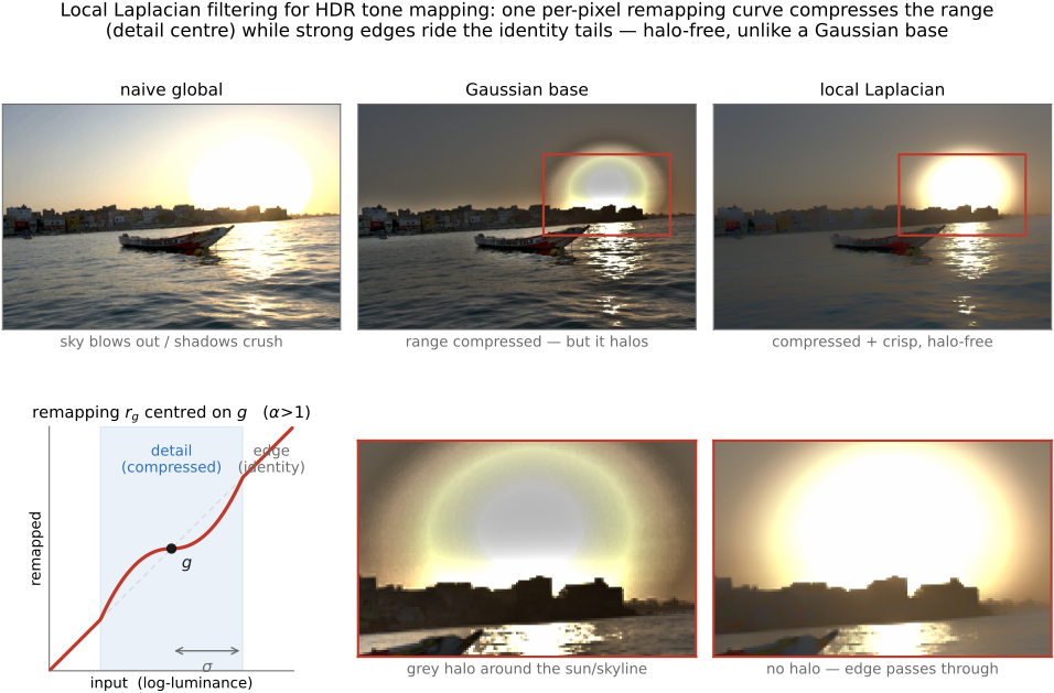
fig-local-laplacian · local Laplacian filters on a real HDR sunset (Paris–Hasinoff–Kautz 2011, implemented from scratch): naive global (blown) vs Gaussian base (halo) vs local Laplacian (halo-free) tone mapping, plus the compressive remapping curve $r_g(\cdot)$ (detail center + identity tails) and a zoom comparison proving the silhouette stays halo-free (Local Laplacian filters) ✅
⬜ figure not yet created
before/after detail-boost with **no halo** fig-wb-before-after
• **start here — Mertens *exposure fusion*, the gentlest pyramid method**: the cleanest way into this chapter is the technique that does **local tone mapping for free, without ever building an HDR image or choosing a tone curve**. Given a **bracketed stack** (or several renderings of one scene), score each pixel of each frame by simple **quality weights** — **contrast** (Laplacian magnitude, "is it sharp here?"), **saturation** (spread of the RGB channels, "is the color alive?"), and **well-exposedness** (closeness to mid-gray, "is it neither crushed nor blown?") — then keep, per pixel, the best-exposed frame. *(Mertens, Kautz & Van Reeth 2007.)* [`fig-exposure-fusion-mertens`]
• **the catch, and the fix — blend in the Laplacian pyramid**: a *per-pixel* weighted average of the frames **seams and halos** (the weights jump at boundaries between which frame "wins"). The fix is **pyramid blending** ([[Pyramids and wavelets]], Burt–Adelson): build a **Laplacian pyramid of each frame** and a **Gaussian pyramid of each (normalized) weight map**, blend the coefficients **level by level** (each frequency band fused at its own scale, with a correspondingly-blurred weight), then collapse. Because every band is feathered over a scale-appropriate transition, the join is invisible and no halos appear — the same reason pyramid blending hides a seam, now driven by exposure-quality weights.
• **why it opens the chapter**: it is the most intuitive instance of the chapter's one idea — *do the edge-aware / local-tone work **band-by-band in a Laplacian pyramid**, not pixel-by-pixel* — and it needs no range weight, no base/detail split, no radiance map. (Full HDR-capture context and where exposure fusion sits among merge-then-tonemap pipelines: [[Multiple exposure imaging]]; here it is the on-ramp to the pyramid machinery.)
• **from fusing a stack to reshaping one image — local Laplacian filters**: exposure fusion *blends several images* in the pyramid; **local Laplacian filters** (Paris et al. 2011) take the same "manipulate the Laplacian pyramid, halo-free" idea and apply it to a **single** image, reshaping its own bands by a pointwise remapping. Same home (the Laplacian pyramid), one input instead of a stack.
• **the odd one out — not an affinity method**: every other technique here weights *pairs* of pixels by similarity; local Laplacian instead works **band-by-band in a Laplacian pyramid** with a **pointwise remapping** — no range weight, no base/detail split (so none of the halos / gradient reversals those can produce). The multiscale cousin of the bilateral, by a different mechanism. Cross-ref [[Pyramids and wavelets]] (the pyramid it's built on) and [[Bilateral filtering]].
• **the mechanism**: to compute the output's Laplacian coefficient at a pixel and level, take the pixel's value $g$, apply a **remapping function** $r_g(\cdot)$ to the *whole* image (a smooth curve, centered on $g$, that decides what is "detail" vs "edge"), build a Laplacian pyramid of that remapped image, and read off **just this level's coefficient at this pixel**; collapse the resulting pyramid for the result.
• **the knob is the remapping $r$**: near $g$ (small amplitude = **detail**) it **compresses or amplifies** — controlling detail / local contrast; far from $g$ (large amplitude = **edge**) it stays the **identity** — so strong edges pass through untouched. One curve → detail enhancement, tone mapping, or inverse tone mapping, all **artifact-free**.
• **why it matters**: state-of-the-art **edge-aware detail manipulation and HDR tone mapping** with no halos and no gradient reversal — the failure modes that motivated the bilateral in the first place.
• **cost & the fast version**: the naive form rebuilds a pyramid per pixel-and-level (expensive); **Aubry et al. 2014** gives a fast approximation and shows the **unnormalized bilateral** is its single-scale relative (ties back to [[Bilateral filtering#Bilateral filter|the unnormalized bilateral]]).
10.4.1 The wish, and why the bilateral leaves a halo⧉
10.4.2 What a Laplacian pyramid hands you⧉
10.4.3 The mechanism: a remapping recomputed per output pixel⧉
10.4.4 One curve, three edits: enhancement, tone mapping, inverse tone mapping⧉
10.4.5 Contrast with the bilateral base/detail split⧉
10.4.6 The cost, and the fast version⧉
▸10.5 Matting Laplacian⧉
10.5.6 Beyond matting: spatially-varying white balance⧉
▸10.6 Guided image filtering⧉
• **the idea**: like the joint bilateral (filter $I$, take structure from a **guide** $J$) but the output is a **local linear transform of the guide**, $I^{\mathrm{out}}=a_k J + b_k$ fit per window by **least squares** — so it preserves the guide's edges by construction
• **why prefer it**: **$O(N)$**, **no range-quantization artifacts** (the gradient reversal the bilateral can show), and **differentiable** → drops into learning pipelines
• **uses**: edge-preserving smoothing; detail enhancement; **flash / no-flash**; **matting / feathering**; **dehazing** (guide = the hazy image — xref He, Sun & Tang 2009 dark-channel, [[#Dehazing as a prior-driven inverse problem]]); depth upsampling
• the affinity is now **implicit** in the local linear fit — same family, different mechanism; a fitting end-point for the chapter's through-line (bilateral → grid → learned → regression → optimization → guided, all *affinity*)
10.6.1 The key idea: the output is a local line in the guide⧉
10.6.2 Fitting the line, and the one knob⧉
10.6.3 Why it is fast: O(N) regardless of window size⧉
10.6.4 No gradient reversal⧉
10.6.5 Reading the affinity back out⧉
10.6.6 Where it is used⧉
▸10.7 Locally adaptive regression kernel (LARK)⧉
• **the view**: treat denoising / upsampling as **local regression** — fit a smooth function to nearby pixels, weighted by a kernel
• **steering / adaptive kernels**: shape the kernel to the **local image structure** — estimate the local gradient, then **stretch the kernel *along* edges and squeeze it *across* them** (an anisotropic, data-dependent weight) so it averages along the edge, not across it
• so LARK is the **regression flavor** of the same affinity idea: the kernel geometry is *derived from* local structure, generalizing the bilateral's scalar range weight to an oriented one
• also a **descriptor**: LARK signatures are used for detection / matching (Seo & Milanfar) — note in passing, not developed
10.7.1 Change the verb: from averaging to fitting⧉
10.7.2 Steering the kernel to the local structure⧉
10.7.3 The regression flavor of the affinity⧉
10.7.4 LARK as a structure descriptor⧉
▸10.8 Poisson image editing⧉
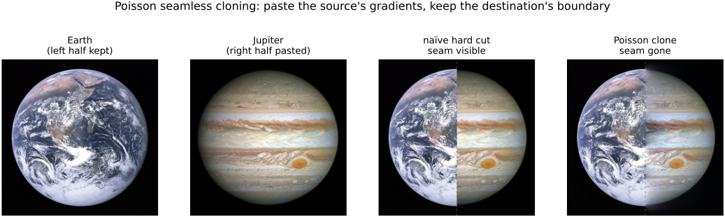
fig-seamless-cloning
fig-seamless-cloning · Poisson seamless cloning (Pérez 2003), EDGES MATTER → Poisson editing: a disk of Jupiter cloned onto Earth — destination (target ring) · source patch · naive paste (visible ring) · Poisson paste (seam gone) ✅
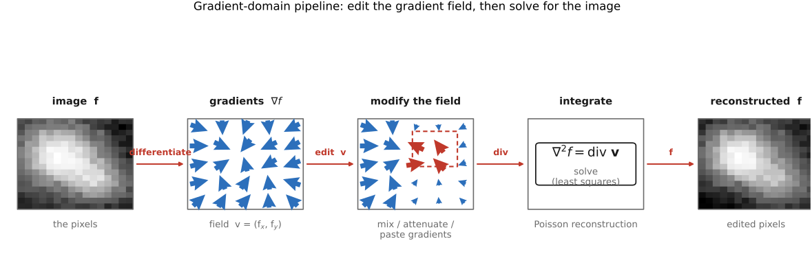
fig-gradient-domain-pipeline
fig-gradient-domain-pipeline · gradient-domain (Poisson) workflow: image → take gradients (∇f) → modify the field → integrate by solving ∇²f=div v → reconstructed (EDGES MATTER → Poisson editing) ✅
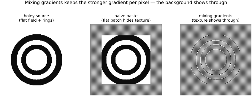
fig-mixing-gradients
fig-mixing-gradients · mixing gradients — keep the per-pixel *stronger* gradient so destination texture shows through holey / transparent inserts (naive vs max-gradient paste) (Poisson editing) ✅
⬜ figure not yet created
`fig-chong-colorspace-results` — results from Chong, Gortler & Zickler 2008 [placeholder] fig-chong-colorspace-results
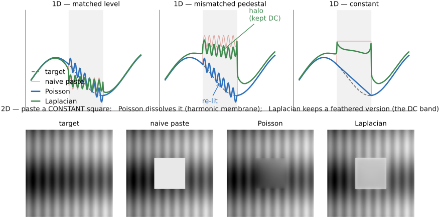
fig-poisson-vs-laplacian-blend
fig-poisson-vs-laplacian-blend · Poisson vs Laplacian-pyramid blending, contrasted on the DC: 1-D three cases (matched level — both agree; mismatched pedestal — Poisson re-lights, pyramid leaves a halo; constant — Poisson ramps/dissolves, pyramid keeps a feathered plateau) + 2-D (paste a constant square — Poisson dissolves it via the harmonic membrane, pyramid keeps a feathered version) ✅
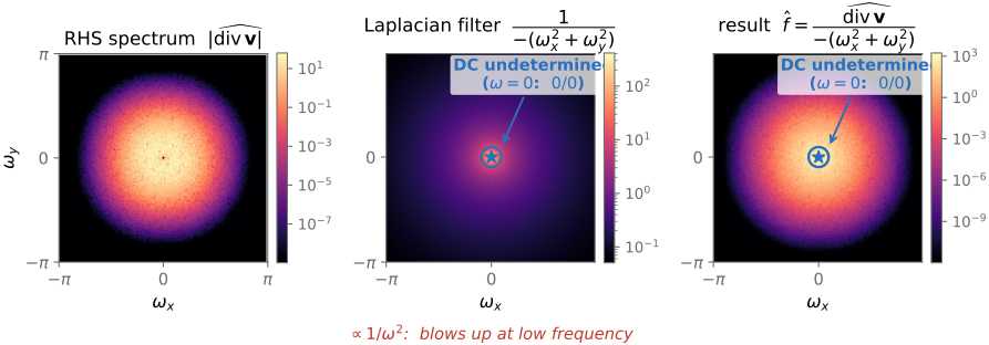
fig-poisson-fourier
fig-poisson-fourier ·
equations
the **Poisson equation** $\nabla^2 f = \operatorname{div}\mathbf{v}$ (reconstruct the field $f$ whose gradient best matches guidance $\mathbf{v}$)
the **discrete Laplacian** system $4f_{p}-\sum_{q\in N(p)} f_{q}=\sum_{q\in N(p)}\!\big(\,v_{pq}\,\big)$ (one sparse equation per pixel $p$ over its 4-neighbors $N(p)$)
the **seamless-cloning Dirichlet boundary condition** $f|_{\partial\Omega}=f^{*}|_{\partial\Omega}$ (interior gradients from the source, boundary values pinned to the destination $f^{*}$)
10.8.4 A perception-based color space⧉
10.8.7 Screened Poisson: pinning the low frequencies⧉
10.8.9 Decolorization (Color2Gray) — keeping isoluminant contrast⧉
▸10.9 Seam optimization⧉
• **the third leg of EDGES MATTER** (the part's framing payoff): Poisson **reconstructs from edges**, bilateral **smooths except across edges**, seam optimization **cuts along edges**. State it as the dual of edge preservation: edge-preserving filtering works *hard to avoid* edges; seam methods *go looking for them* — a transition is invisible exactly where the image is already changing, so we hide the cut **in the edges / busy texture** and keep it **out of smooth regions** where a seam would scream. (Callback to the part intro's "respect the edges.")
• the **unifying machinery**: all three sub-families are **discrete optimization on a graph or grid** — a 1-D least-cost path (**DP**), a 2-D globally-optimal boundary (**graph cut / min-cut**), or a spectral partition (**normalized cuts**). What changes between methods is **the energy / affinity**, not the optimizer.
💡 **Big lesson:** *many image edits are **discrete optimization on a graph** — dynamic programming, min-cut/max-flow, or spectral relaxation — and the **energy (affinity) you choose is the whole game**.* The optimizer is off-the-shelf; **what** you penalize (gradient magnitude, label disagreement across edges, region/boundary cost) is the design. This is the **L4.21 affinity** principle (Bilateral) turned into a *cut*: there the affinity said "average these together"; here it says "**don't cut here**." *(Register as new lesson **L6.4 · Image edits as discrete optimization on a graph (the energy is the design)**, first appearance here; "also relevant": Poisson/photomontage, compositing/segmentation/matting, texture synthesis, stereo/MRF labeling. Full box at this section's head; one-line callback to L4.)*
10.9.5 GrabCut — interactive cutout from a single rectangle⧉
▸10.10 Recap: which edge-aware technique when?⧉
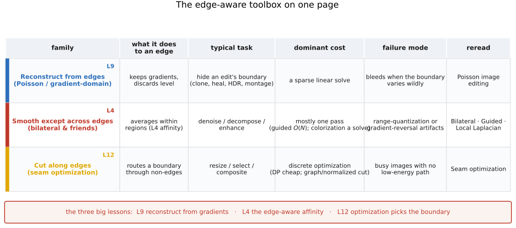
fig-edge-aware-taxonomy
fig-edge-aware-taxonomy ·
10.10.3 A worked chooser⧉