45.26 Interactive demos index and search⧉
The book ships a growing collection of interactive demos (small inline widgets and larger embedded simulators, not counting the xkcd comic embeds). This appendix indexes all of them. Every row, searched or browsed, carries four buttons on its right, and a copy button beside each one so you can hand someone the exact address you are looking at. In book goes to the figure in its chapter, with the explanation around it, and is where the thumbnail and the title point too. The other three put the demo on a page of its own, with nothing around it: on its own here, new tab in a second tab so a lecture can keep one demo per tab, and full screen straight to the projector. Those pages are yours to use in teaching, and they say so: each carries a line crediting the book, which is all the permission you need and all the acknowledgement we ask for.
45.26.1 Find a demo⧉
Naming a field works too. Type "computer vision" or "physically based rendering" and you get the demos of that subject, not the handful whose captions happen to use those words, because the finder matches a field or subject name against the map below before it matches anything against the text.
You can also browse rather than search. Browse by topic opens the whole map: sixty-odd topics, grouped, each with a count of the demos under it. They are not organized the way this book is, on purpose. These demos get used in optics courses, in computer vision, in graphics, in perception, so the topics run from geometric optics and stereo through global illumination and reflectance to cones and displays. Pick as many as you like; pick some and type as well, and the words search inside the topics.
If nothing useful comes back, tell the finder what you were after. Every search is recorded, the words only, so a search that finds nothing is already a request; the box under the results is for saying it in your own words, and for leaving an address if you want an answer. Most of the demos in this book exist because a lecture needed one.
45.26.2 Sharing, linking, and embedding a demo⧉
Every interactive figure carries a small toolbar at the top of the widget:
- 🔗 link copies a deep link straight to that figure.
- 🎚 link+state copies a link that reopens the figure with your current slider and toggle settings. Use it to point someone at a specific configuration, or to embed a figure in a chosen state.
- </> embed (on the standalone simulators) copies an
<iframe>snippet you can paste into your own page.
You can also write the settings into the URL by hand. For an inline widget on a chapter page, add one query parameter per control, named <fig-id>.<control>, before the #<fig-id> anchor; for a standalone simulator page, name the parameters just <control>. Parameters are &-separated and booleans are 1/0. The parameter uses the control’s internal key, which can differ from its visible label. Use the copied state link to obtain the keys. For example:
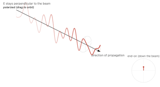
…/sections/02-01-light-and-physics.html?fig-polarization-wave.mode=filter&fig-polarization-wave.dop=0&fig-polarization-wave.pol=90#fig-polarization-waveopens the polarization-wave figure as an analyser at 90° acting on unpolarized light.…/photo101-bounce-flash/index.html?preset=ceiling&ceilPow=0.4&skinMel=0.8opens the bounce-flash simulator bouncing off the ceiling, the ceiling light at 0.4× the flash, with darker skin.
Anything you leave out keeps its default, so you only list what you want to change.
45.26.3 Introduction⧉
- Lattice-focal lens, the result: a lens co-designed with its algorithm: a standard lens holds one plane sharp, while the lattice-focal capture deconvolves to an image sharp throughout. Figure 1.1.3: Chapter 1.1, From digital to computational photography
- When the limitation is the point: a backlit estuary and a long exposure, where accepting what the medium cannot do is the photograph rather than a defect to fix. Figure 1.1.5: Chapter 1.1, From digital to computational photography
- Raw against edited, one frame: the same capture through a flat pipeline and then through a finished edit, so the size of what editing does is visible at full resolution. Figure 1.1.4: Chapter 1.1, From digital to computational photography
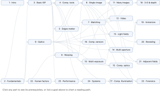 Chapter dependency graph: tick the parts you want to learn; the graph lights up their prerequisites and dims the rest, a personalized reading path. Figure 1.2.1: Chapter 1.2, How to read this book
45.26.4 Fundamentals — light, optics, sensors⧉
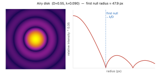 Airy disk: the diffraction-limited PSF of a circular aperture; smaller aperture → bigger disk. Figure 2.1.47: Chapter 2.1, Light and optics
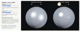 Highlight size: BRDF × light: side by side, blur a highlight by roughening the surface or by enlarging the light; a second point light shows the difference. Figure 2.1.38: Chapter 2.1, Light and optics
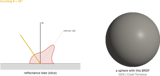 BRDF explorer: pick a reflectance model (Lambertian / Blinn-Phong / GGX), see the lobe and a shaded sphere. Figure 2.1.36: Chapter 2.1, Light and optics
- Cephalopod color, under neural control: a cuttlefish driving pigment and structure at once, which is two of this section's color mechanisms in one animal. Figure 2.1.34: Chapter 2.1, Light and optics
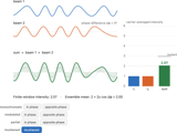 Coherence addition: how two light waves add, coherent versus incoherent. Figure 2.1.10: Chapter 2.1, Light and optics
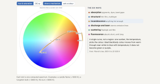 Color mechanism map: pick a mechanism and see which colors it can and cannot reach; every region was computed by pushing real spectra through the color-matching functions, so the boundaries are results rather than drawings. Figure 2.1.29: Chapter 2.1, Light and optics
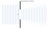 Diffraction vs aperture size: a smaller slit diffracts more; spread angle θ ≈ λ/D. Figure 2.1.45: Chapter 2.1, Light and optics
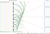 Diffraction grating: A diffraction grating, two ways, sharing geometry and controls (wavelength λ, slit spacing d, and the angle of incidence θ₀). Figure 2.1.17: Chapter 2.1, Light and optics
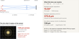 Diffraction limit calculator: what a given aperture can actually resolve. Figure 2.1.48: Chapter 2.1, Light and optics
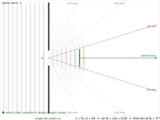 Diffraction single slit: diffraction at a single aperture, two ways (companion to the grating figure). Figure 2.1.16: Chapter 2.1, Light and optics
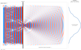 Diffraction wave simulation: live 2-D FDTD wave through a slit; wavefronts bow and spread. Figure 2.1.46: Chapter 2.1, Light and optics
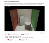 Global illumination: light bounces: a ceiling light fills a room by bouncing (virtual point lights, up to 4 bounces); toggle GI, color-code each point by which bounce lit it, pick a scene, orbit and move. Figure 2.1.44: Chapter 2.1, Light and optics
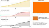 Illumination × reflectance: the color signal is light E(λ) times surface ρ(λ), multiplied wavelength by wavelength. Figure 2.1.28: Chapter 2.1, Light and optics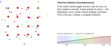
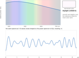
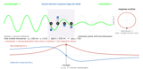 Lorentz resonance: light–matter interaction as driven bound electrons; emergent n(ω) and absorption. Figure 2.1.18: Chapter 2.1, Light and optics
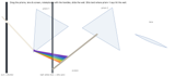 Newton prism puzzle: the same experiment, rebuilt as a puzzle. Figure 2.1.5: Chapter 2.1, Light and optics
- Polarization wave: the transverse E/B fields of a light wave in 3-D, with a phase slider. Figure 2.1.26: Chapter 2.1, Light and optics
- Polarizer over a car hood: the same sunglasses in two orientations, one cutting the glare off the paint and one letting it straight through. Figure 2.1.27: Chapter 2.1, Light and optics
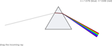 Prism dispersion: white light split by a prism, traced wavelength by wavelength via n(λ). Figure 2.1.15: Chapter 2.1, Light and optics
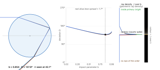 Rainbow droplet: trace rays through a water drop; the rainbow is the caustic at the stationary deviation. Figure 2.1.21: Chapter 2.1, Light and optics
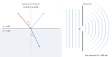 Reflection / refraction / diffraction: the three things light does at a boundary, side by side. Figure 2.1.12: Chapter 2.1, Light and optics
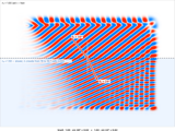 Refraction wave simulation: live 2-D wave crossing into a slower medium; Snell's law emerges. Figure 2.1.14: Chapter 2.1, Light and optics
 Structural color interference: structural color as interfering wavelets. Figure 2.1.32: Chapter 2.1, Light and optics
 Pigment against structural color: an apple colored by absorption beside a beetle and a feather colored by interference, photographed at the same scale. Figure 2.1.30: Chapter 2.1, Light and optics
 cos⁴ falloff: natural vignetting: drag the field angle and watch corner darkening. Figure 2.4.3: Chapter 2.4, Image measurements as integrals over the plenoptic function
 Plenoptic light field (2-D): the light field: a static flatland scene's plenoptic function is the plane. Figure 2.4.4: Chapter 2.4, Image measurements as integrals over the plenoptic function
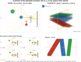 Plenoptic spacetime volume: A portion of the plenoptic function reaching a camera, for a 2-D scene, as a 3-D ray-space-time volume. Figure 2.4.5: Chapter 2.4, Image measurements as integrals over the plenoptic function
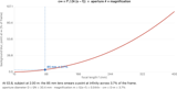 Background blur vs focal length: background blur versus focal length. Figure 2.5.20: Chapter 2.5, Depth of field
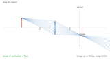 Circle of confusion: a thin lens imaging a point as a ray bundle; focus and aperture shrink the blur disk. Figure 2.5.3: Chapter 2.5, Depth of field
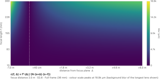 CoC over focal length and defocus: the circle of confusion as a field over focal length and defocus. Figure 2.5.22: Chapter 2.5, Depth of field
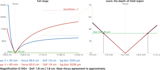 CoC same magnification: two focal lengths at the same magnification. Figure 2.5.18: Chapter 2.5, Depth of field
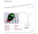 Depth-of-field simulator: a 3-D scene where aperture and focus reshape the depth of field. Figure 2.5.25: Chapter 2.5, Depth of field
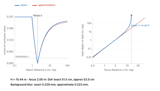 DoF approx vs exact: exact formulas versus their approximations. Figure 2.5.11: Chapter 2.5, Depth of field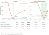
- Depth of field at 1:1: the same macro scene and the same lens, changing only the aperture, where the depth of field is measured in millimeters. Figure 2.5.1: Chapter 2.5, Depth of field
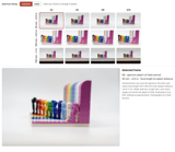 DoF parameter grid: depth of field versus all its parameters. Figure 2.5.12: Chapter 2.5, Depth of field
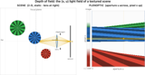 DoF ray space: the light field of a textured scene, and how the aperture integral blurs it. Figure 2.5.26: Chapter 2.5, Depth of field
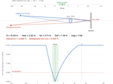 Depth-of-field ray diagram: near/far DoF limits and hyperfocal distance from f, N, subject distance. Figure 2.5.17: Chapter 2.5, Depth of field
- Focus breathing: refocusing a 90 mm lens changes the projected size of the subject, which is why a focus pull is also a small zoom. Figure 2.5.15: Chapter 2.5, Depth of field
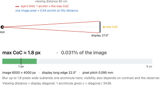 Max CoC calculator: the acceptable circle of confusion, from the viewing conditions. Figure 2.5.5: Chapter 2.5, Depth of field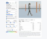
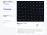
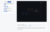
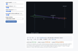
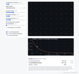
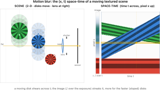 Motion blur space time: the space-time of a moving textured scene, and how the exposure integral streaks it. Figure 2.6.13: Chapter 2.6, Motion blur
- Two kinds of panning: translational panning that follows a rider past the camera, and rotational panning, with what each does to the background. Figure 2.6.6: Chapter 2.6, Motion blur
- Full-spectrum conversion: the magenta IR-cut filter lifted out of a camera, and what the sensor sees once it is gone. Figure 2.7.7: Chapter 2.7, Sensors: photosites, CCD vs CMOS
 Photoelectric effect: the photoelectric effect. Figure 2.7.1: Chapter 2.7, Sensors: photosites, CCD vs CMOS
 Rolling shutter: global vs rolling readout of a moving object; skew and bending. Figure 2.7.11: Chapter 2.7, Sensors: photosites, CCD vs CMOS
 Sensor DoF: sensor size changes depth of field when framing and f-number are held fixed. Figure 2.7.16: Chapter 2.7, Sensors: photosites, CCD vs CMOS
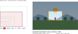 Sensor FOV: sensor size sets field of view. Figure 2.7.15: Chapter 2.7, Sensors: photosites, CCD vs CMOS
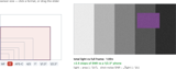 Sensor light: compare sensor size under stated exposure, pixel, and noise assumptions. Figure 2.7.18: Chapter 2.7, Sensors: photosites, CCD vs CMOS
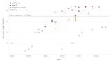 Sensor progress: resolution, dynamic range and low-light of landmark sensors over the years. Figure 2.7.20: Chapter 2.7, Sensors: photosites, CCD vs CMOS
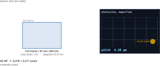 Sensor size explorer: sensor size and photosite size, together. Figure 2.7.13: Chapter 2.7, Sensors: photosites, CCD vs CMOS
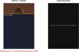 Shutter sync: focal-plane curtains and flash sync banding, slowed way down. Figure 2.7.10: Chapter 2.7, Sensors: photosites, CCD vs CMOS
- A cooled astronomy camera: the bare sensor with no cover glass, the thermoelectric stack behind it, and the parts a photographic camera does not carry. Figure 2.8.2: Chapter 2.8, Noise, signal-to-noise ratio and dynamic range
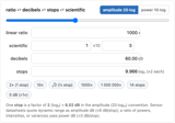 Ratio units converter: decibels, photographic stops, a plain ratio and scientific notation are four ways of writing one multiplicative factor; type into any field and the others follow. Figure 2.8.5: Chapter 2.8, Noise, signal-to-noise ratio and dynamic range
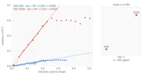 Noise is affine: measured sensor-noise variance is affine in intensity, slope grows with ISO. Figure 2.8.7: Chapter 2.8, Noise, signal-to-noise ratio and dynamic range
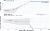 Noise bias curve: measure bias and noise across signal levels. Figure 2.8.11: Chapter 2.8, Noise, signal-to-noise ratio and dynamic range
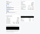 Noise calculator: sensor noise calculator. Figure 2.8.18: Chapter 2.8, Noise, signal-to-noise ratio and dynamic range
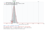 Noise model compare: the fast affine-Gaussian model against the full sensor recipe. Figure 2.8.9: Chapter 2.8, Noise, signal-to-noise ratio and dynamic range
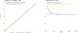 Noise vs ISO: noise as a function of ISO. Figure 2.8.13: Chapter 2.8, Noise, signal-to-noise ratio and dynamic range
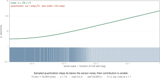 Quantization against noise: set the signal and the read noise and see whether the quantization step is smaller than the noise it has to hide behind, which helps mask banding but does not guarantee invisibility. Figure 2.8.17: Chapter 2.8, Noise, signal-to-noise ratio and dynamic range
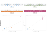 Poisson noise: photon shot noise as a function of photon count. Figure 2.8.1: Chapter 2.8, Noise, signal-to-noise ratio and dynamic range
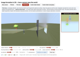 Image formation (3-D), lens: the same experiment in 3-D, on the thick lens: orbit the scene, click the sensor to see the cone of rays one pixel now gathers, and read the recorded image in the inset. Figure 2.3.3: Chapter 2.3, Lens Image formation
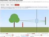 Image formation lens: the 2-D image-formation playground again, opened on the thick lens. Figure 2.3.2: Chapter 2.3, Lens Image formation
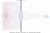 Thick-lens wave simulation: a wave focused by a biconvex glass slab; focusing as emergent physics. Figure 2.3.8: Chapter 2.3, Lens Image formation
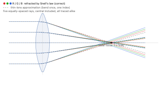 Thin lens approximation: the thin lens is the small-angle linearization of a real, thick, Snell's-law lens. Figure 2.3.9: Chapter 2.3, Lens Image formation
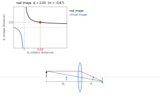 Thin-lens conjugates: the conjugate relation 1/d_o + 1/d_i = 1/f, plotted and drawn. Figure 2.3.12: Chapter 2.3, Lens Image formation
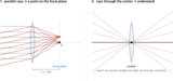 Thin lens two rules: the two thin-lens ray rules (interactive), in the order of the lesson. Figure 2.3.10: Chapter 2.3, Lens Image formation
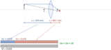 Thin lens: the thin-lens model and its focus equation. Figure 2.3.11: Chapter 2.3, Lens Image formation
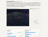 Camera projection: a 3-D scene projected through a pinhole by p ~ K[R|t]X, with live intrinsics/extrinsics. Figure 2.2.17: Chapter 2.2, Pinhole Image Formation and linear perspective
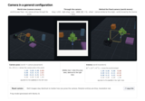 Camera transforms sim: moving the camera equals moving the world by the inverse, in three live 3-D views. Figure 2.2.15: Chapter 2.2, Pinhole Image Formation and linear perspective
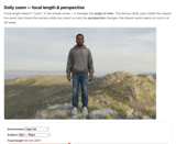 Dolly-zoom simulator: dolly and zoom together to hold the subject while the background rushes. Figure 2.2.23: Chapter 2.2, Pinhole Image Formation and linear perspective
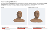 Face-distortion simulator: how focal length and camera distance reshape a face. Figure 2.2.21: Chapter 2.2, Pinhole Image Formation and linear perspective
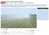 Image formation (3-D): the same idea in 3D. Figure 2.2.4: Chapter 2.2, Pinhole Image Formation and linear perspective
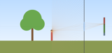 Image formation: which rays reach each point, Big Lesson L2.10 show made playable. Figure 2.2.3: Chapter 2.2, Pinhole Image Formation and linear perspective
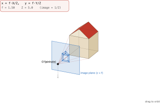 Perspective projection (3-D): perspective projection in 3D. Figure 2.2.13: Chapter 2.2, Pinhole Image Formation and linear perspective
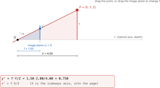 Perspective projection: the perspective projection equation by similar triangles. Figure 2.2.12: Chapter 2.2, Pinhole Image Formation and linear perspective
45.26.5 Visual perception and color⧉
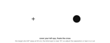 Find your blind spot: cover one eye, fixate the cross and move toward the screen until the target vanishes; the figure turns the on-screen separation into degrees of visual field. Figure 3.1.4: Chapter 3.1, The eye and image formation
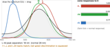 Abnormal cones: how color-vision deficiency reshapes the cones and their responses. Figure 3.2.16: Chapter 3.2, Perceptual color and trichromatic vision
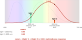 One cone can't tell colors apart: two monochromatic lights auto-scaled to the same response for a chosen cone; univariance made concrete. Figure 3.2.3: Chapter 3.2, Perceptual color and trichromatic vision
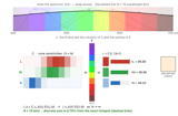 Cone response matrix: cone response as a matrix–vector product. Figure 3.2.5: Chapter 3.2, Perceptual color and trichromatic vision
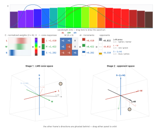 Cones to DKL, on one line: the spectrum meets the cone matrix and then the DKL matrix with every intermediate shown, so the two stages of early color coding read as one pipeline. Figure 3.2.18: Chapter 3.2, Perceptual color and trichromatic vision
- Illuminant metamerism, photographed: two grays printed as a metameric pair, matching under one light and separating under another. Figure 3.2.11: Chapter 3.2, Perceptual color and trichromatic vision
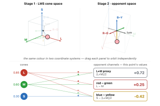 LMS ↔ opponent (3-D): human color in two stages, shown as geometry. Figure 3.2.19: Chapter 3.2, Perceptual color and trichromatic vision
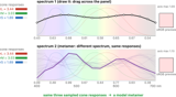 Metamer explorer: build spectra that differ everywhere yet share the same three cone responses and the same perceived color. Figure 3.2.10: Chapter 3.2, Perceptual color and trichromatic vision
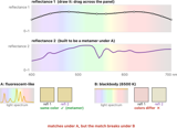 Metamerism illumination: metamerism depends on the light. Figure 3.2.13: Chapter 3.2, Perceptual color and trichromatic vision
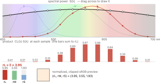 Spectrum → cones: scribble a spectrum and watch the three cones respond; the product-sum that turns a spectrum into three numbers, written out. Figure 3.2.2: Chapter 3.2, Perceptual color and trichromatic vision
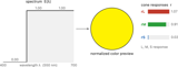 Trichromatic mixer: mix a color from three numbers. Figure 3.2.7: Chapter 3.2, Perceptual color and trichromatic vision
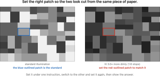 Arend and Reeves, run on you: two patchworks of the same papers under different light; match the marked patch, then watch your answer move when the instruction changes from matching the paper to matching the light. Figure 3.3.5: Chapter 3.3, Adaptation and constancy
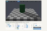 Checker shadow, rendered: Adelson's illusion generated rather than painted, so the equal squares are a consequence of the scene instead of a choice by the artist; orbit it and the illusion holds. Figure 3.3.10: Chapter 3.3, Adaptation and constancy
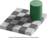 Checker-shadow illusion: Adelson's illusion, with a toggle to the equal-gray proof. Figure 3.3.9: Chapter 3.3, Adaptation and constancy
- Photography reveals the light: scenes where the camera keeps the illumination that the eye works hard to discount. Figure 3.3.14: Chapter 3.3, Adaptation and constancy
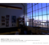 One gain per fixation: move the pointer across a ten-stop radiance map and the display re-exposes for wherever you are looking, which is roughly what the eye does. Figure 3.3.2: Chapter 3.3, Adaptation and constancy
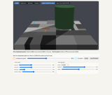 Mondrian shadow match: the matching task run inside a rendered scene with a real soft shadow, so surface and light can be separated by hand. Figure 3.3.11: Chapter 3.3, Adaptation and constancy
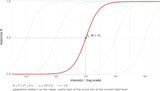 Naka–Rushton response: light adaptation as a sliding response curve. Figure 3.3.1: Chapter 3.3, Adaptation and constancy
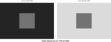 Simultaneous contrast: two squares filled from one number; slide the surrounds apart and the squares separate perceptually while the numbers stay identical. Figure 3.3.7: Chapter 3.3, Adaptation and constancy
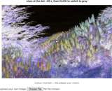 Spanish-castle afterimage: the Spanish-Castle illusion, a demonstration of color adaptation. Figure 3.3.3: Chapter 3.3, Adaptation and constancy
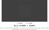 Measure your Weber fraction: lower the increment until the patch disappears; the ratio you land on is your own threshold, measured on your own screen. Figure 3.3.6: Chapter 3.3, Adaptation and constancy
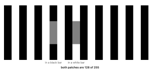 White's illusion: one gray on a square-wave grating, lighter in the black bar than in the white one, which is the way round that simple contrast cannot explain. Figure 3.3.8: Chapter 3.3, Adaptation and constancy
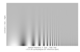 Campbell–Robson chart: see your own contrast sensitivity function drawn by your visual system. Figure 3.4.2: Chapter 3.4, Spatial and temporal vision
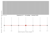 CSF by adjustment: measure your own contrast sensitivity with a row of per-frequency sliders. Figure 3.4.3: Chapter 3.4, Spatial and temporal vision
- Acuity, eagle to jumping spider: the sharpest and the coarsest eyes known, put on one scale. Figure 3.6.9: Chapter 3.6, Animal eyes
- Seeing in air and water: five real strategies for forming an image across the boundary, one per approach the section describes. Figure 3.6.6: Chapter 3.6, Animal eyes
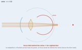 Amphibious eyes ray-trace: the problem, and five ways around it, for seeing in both air and water, traced as rays through a schematic eye (cornea + lens + retina). Figure 3.6.5: Chapter 3.6, Animal eyes
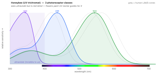 Animal cone curves: photoreceptor spectral sensitivities across the animal kingdom. Figure 3.6.13: Chapter 3.6, Animal eyes
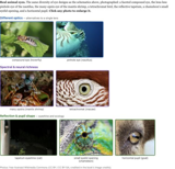 Animal eyes, photographed: the companion to the schematic designs, close enough to see the pupil, the tapetum and the shape of the lens. Figure 3.6.3: Chapter 3.6, Animal eyes
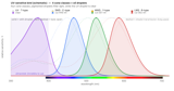 Animal oil droplets: colored oil droplets: a color-filter array grown one droplet per cone. Figure 3.6.14: Chapter 3.6, Animal eyes
- Eyes in front or on the side: a predator's forward pair against a prey animal's lateral pair, and the trade of binocular overlap against field of view. Figure 3.6.7: Chapter 3.6, Animal eyes
- Three tricks for scarce light: a reflective tapetum, a wide pupil and a slow integration time, each on the animal that uses it. Figure 3.6.8: Chapter 3.6, Animal eyes
- Pupil shapes and the lives they fit: slits, circles and the goat's horizontal bar, each labeled with the advantage it buys. Figure 3.6.4: Chapter 3.6, Animal eyes
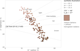
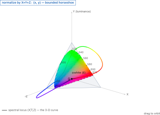 Chromaticity (3-D): the chromaticity diagram as a flat cross-section of Koenderink's 3-D cone, orbitable. Figure 4.1.8: Chapter 4.1, Color space 101
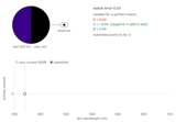 Color-matching experiment: turn three primary knobs to match a test light; trace the color-matching functions. Figure 4.1.5: Chapter 4.1, Color space 101
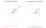 Dual basis reconstruction: reconstruction in a non-orthogonal basis, wrong and right. Figure 4.1.4: Chapter 4.1, Color space 101
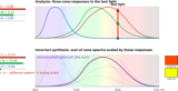 Incorrect synthesis: why the cone curves are the wrong synthesis primaries. Figure 4.1.3: Chapter 4.1, Color space 101
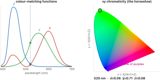 LMS horseshoe: the chromaticity horseshoe in LMS cone space, and where its shape comes from. Figure 4.1.9: Chapter 4.1, Color space 101
45.26.6 Color spaces and color technology⧉
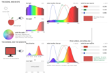 Color reproduction end to end: a lamp multiplied by a reflectance and projected onto three cone sensitivities, then reproduced on a display, with every stage editable. Figure 4.1.1: Chapter 4.1, Linear color reproduction and CIE XYZ
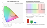 What spectrum makes this color: drag a point anywhere on the chromaticity diagram, including outside the horseshoe, and see the spectrum that would produce it or why none can. Figure 4.1.10: Chapter 4.1, Linear color reproduction and CIE XYZ
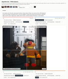 Relight a hyperspectral scene: every pixel carries a full reflectance spectrum, so the scene can be rendered under any illuminant and the white balance judged against the truth. Figure 4.2.9: Chapter 4.2, White balance and white point
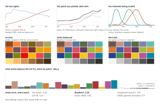 How well white balance works: one gain per channel can only approximate an illuminant change; measure the error on 24 ColorChecker patches, in several bases. Figure 4.2.7: Chapter 4.2, White balance and white point
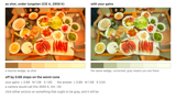 White balance is three numbers: relight the book's own raw files from D65 to any named illuminant with a von Kries transform, and set the three gains yourself. Figure 4.2.1: Chapter 4.2, White balance and white point
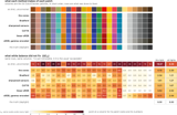 Every patch against every method: a column per surface and a row per treatment, so a method's failures show up as a stripe instead of disappearing into an average. Figure 4.2.8: Chapter 4.2, White balance and white point
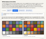 White balance / metamerism: correct a color cast; diagonal vs 3×3, with ΔE. Figure 4.2.6: Chapter 4.2, White balance and white point
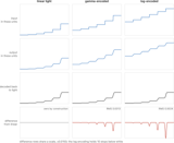 One filter, three encodings: filter a signal in light, in gamma and in log, then decode all three back to light, which is the only place the answers can be compared. Figure 4.3.11: Chapter 4.3, Encoding: linear, gamma or log
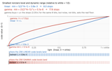 Encoding dynamic range: dynamic range from a bit budget, and why noise undercuts it. Figure 4.3.5: Chapter 4.3, Encoding: linear, gamma or log
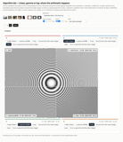 Where the arithmetic happens: ten operations, each run in light, gamma and log over one photograph and displayed identically, so only the space differs. Figure 4.3.12: Chapter 4.3, Encoding: linear, gamma or log
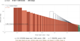 Just-noticeable differences per code step: how many visible steps one code value is worth at each level, which is what decides whether an encoding bands. Figure 4.3.2: Chapter 4.3, Encoding: linear, gamma or log
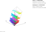 Luma is not luminance: the sRGB gamut cut into sheets of equal luminance and of equal luma, so the shape of the difference is visible rather than asserted. Figure 4.3.6: Chapter 4.3, Encoding: linear, gamma or log
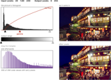 Photoshop 1.0 Levels, live: the 1990 Levels map running from our line-by-line port: black point, white point, and the gamma slider that is not the display gamma. Figure 4.3.7: Chapter 4.3, Encoding: linear, gamma or log
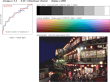 Gamma + quantization banding: storage gamma and bit depth vs shadow banding, on ramp, gradient and photo. Figure 4.3.1: Chapter 4.3, Encoding: linear, gamma or log
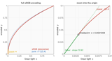 SRGB gamma curve: the piecewise sRGB encoding, up close. Figure 4.3.4: Chapter 4.3, Encoding: linear, gamma or log
 Optimal reflectance: the brightest reflectance that can make a given color. Figure 4.4.6: Chapter 4.4, RGB color spaces
 Color space atlas: one space drawn twice, in its own geometry and in a space that measures, so a cube, a cone and a perceptual box can be compared. Figure 4.5.9: Chapter 4.5, Advanced color: opponents, perceptually-uniform, and preferred
 HSV and HSL are the RGB cube: slice either space and watch the familiar cone or bi-cone come apart into the cube it was made from. Figure 4.5.4: Chapter 4.5, Advanced color: opponents, perceptually-uniform, and preferred
 The picker, and what it hides: drag inside the square and along the hue strip; switching HSV to HSL changes what the square means and which colors it can reach. Figure 4.5.5: Chapter 4.5, Advanced color: opponents, perceptually-uniform, and preferred
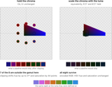 Luma and chroma do not come apart: one Y'CbCr slice at the luma you set, with sample colors carried down by the two rules a codec might use. Figure 4.5.1: Chapter 4.5, Advanced color: opponents, perceptually-uniform, and preferred
- Autochrome, a color filter array in film: dyed starch grains doing Bayer's job a century early, with the screen and the resulting plate side by side. Figure 4.6.7: Chapter 4.6, Sensing color: multiplexing strategies
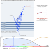 Inside a dichroic coating: the beam splitter cut down to a handful of layers, so the interference that separates the colors is visible layer by layer. Figure 4.6.9: Chapter 4.6, Sensing color: multiplexing strategies
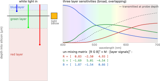 Foveon depth stack: silicon absorption by depth and the Foveon's overlapping color channels. Figure 4.6.17: Chapter 4.6, Sensing color: multiplexing strategies
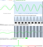 Lippmann standing wave: the standing wave behind Lippmann photography (interactive, 1-D). Figure 4.6.23: Chapter 4.6, Sensing color: multiplexing strategies
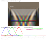 Nano prism demo: design your own nano-prism. Figure 4.6.14: Chapter 4.6, Sensing color: multiplexing strategies
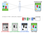 Temporal multiplex plates: color multiplexing in time, following Maxwell's 1861 experiment. Figure 4.6.3: Chapter 4.6, Sensing color: multiplexing strategies
- A trichroic prism: the physical counterpart to the three-sensor diagram, splitting white light into three paths. Figure 4.6.11: Chapter 4.6, Sensing color: multiplexing strategies
- 3-CCD prism rays: the 3-CCD prism's light paths, traced on the real block. Figure 4.6.12: Chapter 4.6, Sensing color: multiplexing strategies
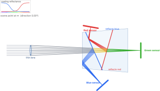 3-CCD prism: the trichroic (3-CCD) prism (interactive ray trace). Figure 4.6.10: Chapter 4.6, Sensing color: multiplexing strategies
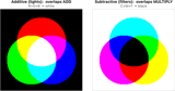 Additive subtractive: additive and subtractive synthesis side by side. Figure 4.7.4: Chapter 4.1, Color space 101
 Gamma probe for your screen: a one-pixel checker against a flat patch measures the whole chain between the number and the light you actually see. Figure 4.3.3: Chapter 4.7, Synthesizing color
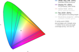 Display gamuts, toggled: sRGB, P3, Rec.2020 and the rest on the chromaticity diagram from published primaries; switch any of them on or off. Figure 4.7.5: Chapter 4.7, Synthesizing color
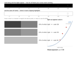 Measure your display response: three matches give the product of everything between code value and light: the browser, the compositor and the panel. Figure 4.7.11: Chapter 4.7, Synthesizing color
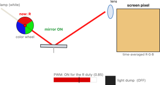 DMD tech: how a DLP projector's micromirror makes a color. Figure 4.7.8: Chapter 4.7, Synthesizing color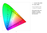
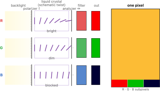
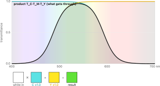 Subtractive spectra: subtractive mixing is multiplication. Figure 4.7.3: Chapter 4.1, Color space 101
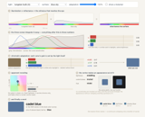 One light to one word: pick an illuminant and a reflectance, and the figure runs all six steps from the spectrum to a color name. the figure: Chapter 4.9, Color TLDR
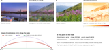 Cross-fade in three spaces: fade two photographs in sRGB code values, in light, and in a perceptual space, and watch colors appear that are in neither photograph. the figure: Chapter 4.9, Color TLDR
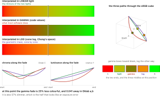 Why gamma fading invents colors: the same two colors faded three ways and plotted as trajectories, so the detour the gamma path takes is visible. the figure: Chapter 4.9, Color TLDR
45.26.7 Photography⧉
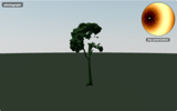 Polarizer on foliage: rotate a polarizer under a simulated polarized sky and watch the sky-colored specular veil come off the leaves. Figure 5.3.8: Chapter 5.3, Viewpoint, lenses, and focus
- Aperture against depth of field: the same portrait wide open and stopped down, the background going from wash to detail. Figure 5.2.2: Chapter 5.2, Exposure and capture timing
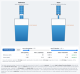 Exposure bucket analogy: the faucet-and-bucket exposure analogy. Figure 5.2.1: Chapter 5.2, Exposure and capture timing
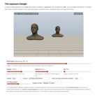 Exposure-triangle simulator: aperture, shutter and ISO trade off for similar output brightness, with different effects on captured light. Figure 5.2.6: Chapter 5.2, Exposure and capture timing
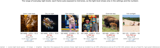 One frame per rung of light: six of the author's own photographs ordered from the darkest scene to the brightest. Figure 17.2.4: Chapter 5.2, Exposure and capture timing
- Where 18% gray fails: the meter renders the average scene to mid-gray, which is wrong for snow and wrong for a black cat. Figure 5.2.7: Chapter 5.2, Exposure and capture timing
- Shutter speed against motion: a child frozen at 1/3200 s and the same subject smeared, with the speed marked on each frame. Figure 5.2.3: Chapter 5.2, Exposure and capture timing
- What the f-number is, physically: an aperture ring running to f/0.95 and the diaphragm behind it, next to a slow lens for scale. Figure 5.3.2: Chapter 5.3, Viewpoint, lenses, and focus
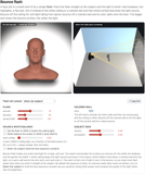
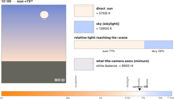 Color temp time: daylight is the warm sun plus the cool sky. Figure 5.4.1: Chapter 5.4, Working with light
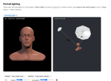 Portrait-lighting simulator: move the key light and shape a portrait. Figure 5.4.5: Chapter 5.4, Working with light
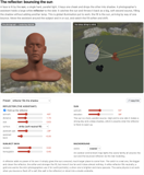 Reflector: bouncing the sun: a white reflector held by an assistant catches the sun and fills the shadow, global illumination in one bounce; orbit the setup view. Figure 5.4.4: Chapter 5.4, Working with light
 Natural illumination (physical sky): a figure under a Preetham sky; set sun azimuth/elevation and turbidity, and reveal the sky's many-point-light approximation. Figure 5.4.2: Chapter 5.4, Working with light
 Four photographs, three renderings: our pipeline, the camera's own render and a reference developer, any two of them across a draggable divider. Figure 5.5.4: Chapter 5.5, Developing and editing a photograph
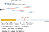 Display acuity calculator: distance, size, resolution, and acuity (interactive calculator). Figure 5.6.1: Chapter 5.6, Preparing photographs for viewing
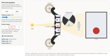 Movie projector: an old-style film projector run frame by frame: intermittent claw pull-down, the Maltese-cross dwell, and the shutter's double flash that beats flicker. Figure 30.1.8: Chapter 5.6, Preparing photographs for viewing
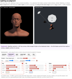 Lighting AS judgment: lighting is never neutral: relight one 3-D face and watch the verdict change. Figure 5.8.20: Chapter 5.8, Photographic representation and its limits
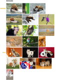 Animal genres: wildlife in the field and pets at home, both uncooperative, fast and shot at eye level. Figure 5.7.11: Chapter 5.7, Photographic situations and tradeoffs
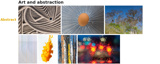 Art and abstraction: images built from form, color, texture and negative space rather than from a named subject. Figure 5.7.15: Chapter 5.7, Photographic situations and tradeoffs
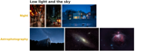 Low light and the sky: night scenes holding lit signage against dark sky, and astrophotography pulling faint detail out of it. Figure 5.7.13: Chapter 5.7, Photographic situations and tradeoffs
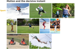 Motion and sport: a fast subject at a distance with one decisive instant, which is the whole problem in one frame. Figure 5.7.1: Chapter 5.7, Photographic situations and tradeoffs
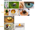 The arranged frame: macro at life size, food styled before it wilts, and still life composed from scratch. Figure 5.7.9: Chapter 5.7, Photographic situations and tradeoffs
 People genres: portraits, a newborn, a concert under colored stage light, one labeled row each. Figure 5.7.3: Chapter 5.7, Photographic situations and tradeoffs
 Places genres: landscapes at the edges of the day, architecture with controlled verticals, and interiors. Figure 5.7.6: Chapter 5.7, Photographic situations and tradeoffs
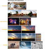 Genres defined by technique: panoramas past a single frame's field of view, light painting, and the rest of the apparatus-led genres. Figure 5.7.17: Chapter 5.7, Photographic situations and tradeoffs
45.26.8 Linear methods and Fourier analysis⧉
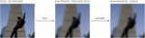 Aliasing prefilter: prefilter before sampling to suppress frequencies that would alias. Figure 6.1.6: Chapter 6.1, Introduction to forward and inverse linear methods
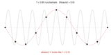 Aliasing (1-D sine): sample a sine past Nyquist and watch it alias to a low frequency. Figure 6.4.1: Chapter 6.1, Introduction to forward and inverse linear methods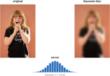
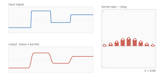 1-D convolution: build a kernel with tap sliders and watch the output update live. Figure 6.2.3: Chapter 6.2, Convolution
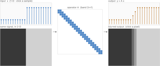 Blur as a matrix: drag a scanline through a photo and watch the banded operator blur it, in one dimension and two. Figure 6.1.2: Chapter 6.1, Introduction to forward and inverse linear methods
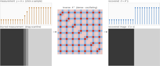 Deblurring, noise-free: invert the same matrix on a clean measurement and get the signal back exactly. Figure 6.1.3: Chapter 6.1, Introduction to forward and inverse linear methods
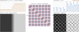 Deblurring, with noise: add a little noise to the measurement and hover a recovered sample to see the inverse amplify it. Figure 6.1.4: Chapter 6.1, Introduction to forward and inverse linear methods
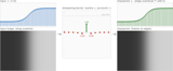 Sharpening as a matrix: the sharpening counterpart, a draggable scanline and its operator side by side. Figure 6.2.16: Chapter 6.2, Convolution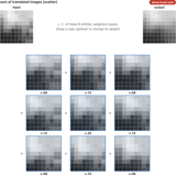
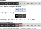 Convolution slide (1-D): convolution in 1-D: a 3-tap kernel sliding along a row of pixels. Figure 6.2.1: Chapter 6.2, Convolution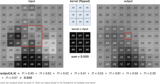
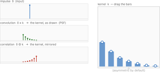
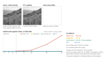 FFT against direct convolution: both timed in your own browser as the figure draws, so the crossover is a measurement on your machine rather than a model of one. Figure 6.3.29: Chapter 6.3, Fourier
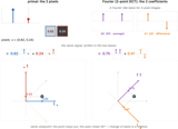 Fourier: two pixels: the 2-pixel example, laid out like the 3-pixel one below. Figure 6.3.6: Chapter 6.3, Fourier
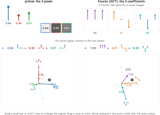 Fourier: three pixels (3-D): A three-pixel image as a point in 3-D, and the DCT as a rotation of the axes. Figure 6.3.7: Chapter 6.3, Fourier
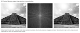 Fourier filtering: draw in the frequency domain and see the spatial result. Figure 6.3.18: Chapter 6.3, Fourier
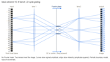 Fourier optics plane: A schematic 4f bench where the lens does the transform. Figure 6.3.26: Chapter 6.3, Fourier
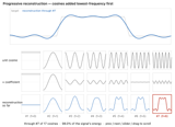 Fourier progressive (1-D): building a 1-D signal one cosine at a time. Figure 6.3.12: Chapter 6.3, Fourier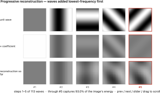
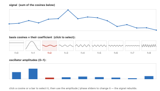 Fourier synthesis (1-D): A 1-D signal is a sum of weighted, phase-shifted cosines. Figure 6.3.10: Chapter 6.3, Fourier
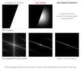 Fourier windowing: spectral leakage and why a Hann/Blackman window cleans up a measured spectrum. Figure 6.3.27: Chapter 6.3, Fourier
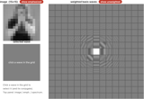 Image fourier synthesis: an image is the sum of weighted sine waves. Figure 6.3.11: Chapter 6.3, Fourier
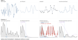 1-D sampling pipeline: signal → prefilter → sample → reconstruct, with continuous spectra and replicas. Figure 6.4.5: Chapter 6.4, Sampling, downsampling, and aliasing
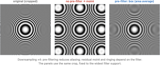 2-D downsampling & moiré: downsample a zone plate with vs without a prefilter. Figure 6.4.6: Chapter 6.4, Sampling, downsampling, and aliasing
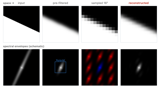 2-D sampling pipeline: the 2-D analog, image and Fourier magnitude side by side. Figure 6.4.7: Chapter 6.4, Sampling, downsampling, and aliasing
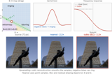 Mitchell–Netravali cubics: the B-C cubic family: kernel, frequency response and test patterns. Figure 6.5.10: Chapter 6.5, Resampling and upsampling
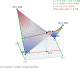 Bilinear height-field: drag four corners and watch the bilinear saddle deform. Figure 6.5.5: Chapter 6.5, Resampling and upsampling
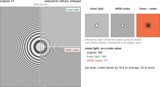 Downsample on light or on code: the same shrink done twice, once averaging sRGB code values and once averaging light, on a pattern built to show the difference. Figure 6.5.17: Chapter 6.5, Resampling and upsampling
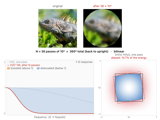 Rotation resample challenge: rotate in many small steps and watch resampling damage compound. Figure 6.5.16: Chapter 6.5, Resampling and upsampling
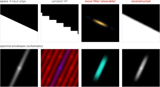 Steered reconstruction: aim an anisotropic filter along an undersampled edge to reconstruct it cleanly. Figure 6.5.19: Chapter 6.5, Resampling and upsampling
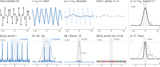 Resampling pipeline in 1-D: samples, reconstruction with k, prefilter h_q and output samples at spacing q, each with its spectrum, and the combined kernel ρ = k ∗ h_q that follows k when enlarging and h_q when shrinking. Figure 6.5.8: Chapter 6.5, Resampling and upsampling
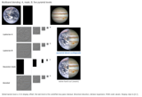 Pyramid blend, step by step: Burt–Adelson multiband blending laid out level by level. Figure 6.6.8: Chapter 6.6, Pyramids and wavelets
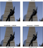 Chapter 6.7, fig-deconv-gamma-linear: why deblurring must be done in linear light (gamma and blur don't commute). Figure 6.8.1: Chapter 6.7, When linearity breaks down
45.26.9 Probabilistic approaches and machine learning⧉
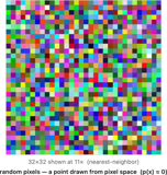 Random vs natural: most arrays of numbers do not look like images. Figure 7.1.2: Chapter 7.1, Imaging as Bayesian inference with probabilistic priors
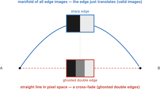 Manifold interpolation: interpolate on the image manifold vs the ambient cross-fade (the "dull average"). Figure 7.1.5: Chapter 7.1, Imaging as Bayesian inference with probabilistic priors
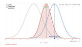 Bayes inference (1-D): an interactive one-dimensional Bayesian-inference demo: drag the data, pick a prior and a likelihood, and compare the posterior, maximum-likelihood estimate, MAP estimate and posterior mean. Figure 7.1.8: Chapter 7.1, Imaging as Bayesian inference with probabilistic priors
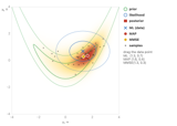 Bayes inference (2-D): the same picture in a two-dimensional parameter space: a prior times an anisotropic, axis-aligned Gaussian likelihood with independently adjustable measurement scales. Figure 7.1.9: Chapter 7.1, Imaging as Bayesian inference with probabilistic priors
 Toy diffusion: forward/reverse diffusion on a 2-D toy distribution (denoising along the score). Figure 7.4.4: Chapter 7.4, Generative AI and diffusion
 Diffusion demo: live diffusion as iterated denoising (simulated, with an optional real Stable Diffusion download). Figure 7.4.11: Chapter 7.4, Generative AI and diffusion
45.26.10 Basic image processing and the ISP⧉
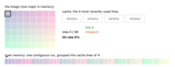 Cache loop order: loop order and the cache, step by step. Figure 8.1.9: Chapter 8.1, Image representation
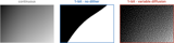 Dithering methods: hide banding as noise: no dither vs stochastic vs Ostromoukhov error diffusion. Figure 8.1.5: Chapter 8.1, Image representation
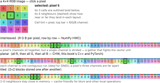 Interleaved against planar: the same RGB row packed both ways with the SIMD load drawn over it, which is why one layout is faster to brighten a channel. Figure 8.1.8: Chapter 8.1, Image representation
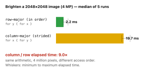 Loop order benchmark: the same slowdown, measured live. Figure 8.1.7: Chapter 8.1, Image representation
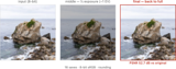 Repeated quantization: how 8-bit rounding accumulates under repeated exposure edits; dither breaks it up. Figure 8.1.4: Chapter 8.1, Image representation
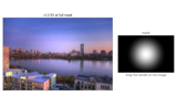 Local point operations: digital dodge and burn: a point op applied through a mask. Figure 8.3.10: Chapter 8.3, Tone point operations
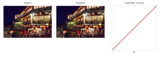 Point operations: per-pixel exposure/contrast/gamma/saturation with a live transfer curve. Figure 8.3.1: Chapter 8.3, Tone point operations
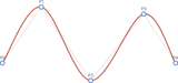 Splines: drag control points and compare spline families (Bézier, Catmull-Rom, B-spline, …). Figure 8.3.9: Chapter 8.3, Tone point operations
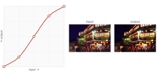 Tone curve: a "Curves"-style tool; drag points to remap an image in real time. Figure 8.3.8: Chapter 8.3, Tone point operations
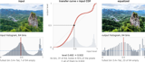 Histogram equalization: the CDF as the tone curve on synthetic and real inputs, discrete or interpolated, with a probe that follows one gray level through it. Figure 8.7.5: Chapter 8.7, Histograms
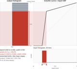 Why the CDF equalizes: drag a band of input levels through the CDF and see it land on an output interval as wide as its share of the pixels; continuous versus discrete bins. Figure 8.7.4: Chapter 8.7, Histograms
 Beauty-curve playground: drag the tone curve; the image stays scene-linear, only the display transform moves. Figure 8.4.2: Chapter 8.4, Beauty curves: the camera "look"
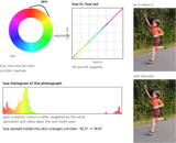 Three hue corridors: sky, vegetation and skin picked out by hue with a half-width each, and the two moves the look applies inside them. Figure 8.6.1: Chapter 8.6, Color beautification and preferred colors
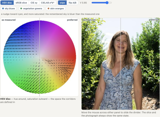 Where the look moves your pixels: the color stage drawn as a vector field, each arrow running from a color to wherever the stage sends it. Figure 8.6.2: Chapter 8.6, Color beautification and preferred colors
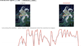 Unsharp masking: linear sharpening and its non-linear halo fixes, with a scanline. Figure 8.8.6: Chapter 8.8, Sharpening
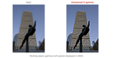 Sharpen in which space?: gamma vs linear vs log for the unsharp mask, and the halos each gives. Figure 8.8.4: Chapter 8.8, Sharpening
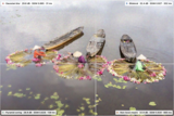 Denoising lab: nine classic filters (Gaussian to NL-means and total variation) in a mouse-driven four-way split, with sliders, PSNR and SSIM, and error views. Figure 13.3.7: Part 13, Denoising
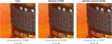 Denoise color harder: split luma/chroma and filter chroma harder to kill color blotches. Figure 13.3.5: Part 13, Denoising
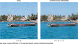 Pyramid (wavelet coring) denoise: per-band soft-threshold sliders on a Laplacian pyramid. Figure 13.4.6: Part 13, Denoising
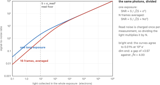 Splitting light is free only in bright light: one photon budget spent as a single long exposure or as the average of N short frames, plotted against how much light the scene delivers. Figure 13.2.9: Part 13, Denoising
 Demosaicking lab: eight classic demosaickers (nearest to AHD) in a mouse-driven four-way split, with sliders, PSNR and SSIM, and error views. Figure 15.2.1: Part 15, Demosaicking and joint methods
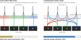 Filtering against routing color: a Bayer quad that throws two thirds of the light away, beside a router that sends each band to a site instead. Figure 15.12.3: Part 15, Demosaicking and joint methods
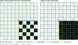 Edge-directed green: how demosaicking picks its two green neighbors along the edge. Figure 15.1.7: Part 15, Demosaicking and joint methods
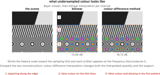 Demosaicking artifact zoo: zippering, false color and the maze, each produced on a synthetic target and zoomed until it is unmistakable. Figure 15.1.6: Part 15, Demosaicking and joint methods
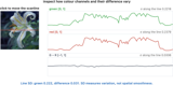 Color differences are smooth: the red and green channels of a photograph beside their difference, which varies far less, and where that assumption breaks. Figure 15.1.10: Part 15, Demosaicking and joint methods
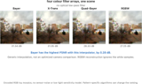 Color filter arrays compared: Bayer, X-Trans, Quad-Bayer and RGBW, each with its pattern, the measured spectrum of its mosaic and a reconstruction. Figure 15.5.2: Part 15, Demosaicking and joint methods
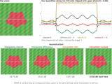 What to interpolate: one scanline across a color boundary: the channel, the color difference, the ratio and the residual against a guide, and which of them stays smooth. Figure 15.2.7: Part 15, Demosaicking and joint methods
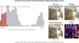 Hard cases for demosaicking: the PSNR distribution of many crops under classical demosaicking, and the thin tail of fine repetitive texture a learned model is trained on. Figure 15.6.1: Part 15, Demosaicking and joint methods
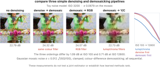 Joint against sequential: one noisy raw crop through three sequential pipelines at matched strength, with the truth and an error map for each. Figure 15.8.2: Part 15, Demosaicking and joint methods
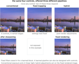 Where the controls live: a conventional pipeline with its parameters, a fixed end-to-end mapping with none, and a hybrid between them. Figure 15.9.1: Part 15, Demosaicking and joint methods
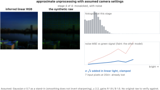 Unprocessing a photograph: a finished photograph stepped back through an approximate inverse pipeline to a noisy synthetic mosaic, one stage at a time. Figure 15.11.1: Part 15, Demosaicking and joint methods
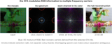 The spectrum of a mosaic: the luminance band and the chrominance copies of a mosaicked image, placed from the array's own tile, for smooth and detailed scenes. Figure 15.3.2: Part 15, Demosaicking and joint methods
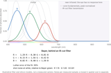 What each sensor measures: the spectral sensitivities of Bayer filters, Foveon's depth layers and an RGB-NIR array on one axis, with the cone fundamentals behind them. Figure 15.12.2: Part 15, Demosaicking and joint methods
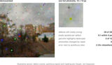 Raw-stage defects: defective photosites and autofocus pixels on a raw crop, with a switch for each correction and a measure of how far one bad sample spreads. Figure 15.7.1: Part 15, Demosaicking and joint methods
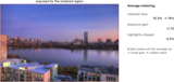 Auto-exposure metering: average / center-weighted / spot metering on the same scene. Figure 8.10.1: Chapter 8.10, Auto-exposure and auto white balance
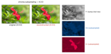 Chroma subsampling: 4:4:4 vs 4:2:2 vs 4:2:0 on a real photo; saturated color edges bleed while luma survives. Figure 8.11.5: Chapter 8.11, File formats and compression
 EXIF explorer: drop in a JPEG, TIFF or raw file and read what it says about the camera, the exposure, the moment and sometimes the place. Figure 8.11.1: Chapter 8.11, File formats and compression
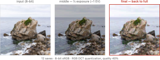 Exposure round-trip (JPEG): 8-bit banding and JPEG generation loss compounding over repeated edits. Figure 8.11.12: Chapter 8.11, File formats and compression
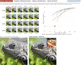 Modern formats, measured: our own encodes of our own photographs, so the size and quality numbers can be checked rather than quoted. Figure 8.11.15: Chapter 8.11, File formats and compression
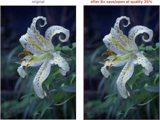 JPEG generation loss: repeatedly saving a JPEG; blocking and ringing compound. Figure 8.11.11: Chapter 8.11, File formats and compression
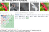 JPEG, stage by stage: a 32×32 color image run through baseline JPEG in five stages (Y′CbCr, 4:2:0, 8×8 DCT, quantization at a chosen quality, zig-zag run lengths and Huffman bits), with one block's numbers at every step, the bit count and the decoded PSNR. Figure 8.11.3: Chapter 8.11, File formats and compression
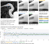 JPEG deblocking: a JPEG coded in the browser and deblocked three ways (boundary filter, projection onto the quantization intervals, a denoiser at σ_q), with PSNR and one block's coefficients against their intervals. Figure 8.11.13: Chapter 8.11, File formats and compression
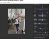 Mini-Lightroom: a real per-pixel raw-develop pipeline driven by a Lightroom-style panel. Figure 8.12.4: Chapter 8.12, Recap ISP, non-destructive editing
45.26.11 Making computational-photography code fast⧉
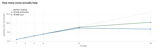 Machine cores: throughput against thread count for cache-resident arithmetic and for streaming, which is how many cores actually help. Figure 29.2.11: Chapter 29.2, Modern CPUs: memory hierarchy, parallelism, and what it takes to go fast
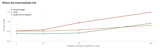 Machine fusion: a four-stage chain with image-sized, cache-sized and register-only intermediates, on one thread and then on every core. Figure 29.2.7: Chapter 29.2, Modern CPUs: memory hierarchy, parallelism, and what it takes to go fast
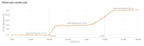 Machine cache latency: a pointer chase from 8 KB to 96 MB: the plateaus are the reader's cache levels and the steps are their capacities. Figure 29.2.4: Chapter 29.2, Modern CPUs: memory hierarchy, parallelism, and what it takes to go fast
 Machine access pattern: 16 MB of pixels summed along rows, down columns and scattered, timed live: identical arithmetic, several-fold difference. Figure 29.2.5: Chapter 29.2, Modern CPUs: memory hierarchy, parallelism, and what it takes to go fast
 Machine probe: the whole chapter measured on the reader's own processor: seven panels behind tabs, from what the browser reports to cache hierarchy, access-pattern cost, fusion, roofline, SIMD gain and the concurrency exposed to the browser. Figure 29.2.13: Chapter 29.2, Modern CPUs: memory hierarchy, parallelism, and what it takes to go fast
 Machine report: the few facts a browser will volunteer about the processor, each with its caveat, and the note that cache sizes and vector width are not among them. Figure 29.2.1: Chapter 29.2, Modern CPUs: memory hierarchy, parallelism, and what it takes to go fast
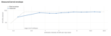 Machine roofline: the reader's own compute roof, streaming bandwidth and ridge point, swept by doing a controlled number of multiply-adds per byte streamed. Figure 29.2.9: Chapter 29.2, Modern CPUs: memory hierarchy, parallelism, and what it takes to go fast
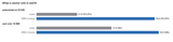 Machine SIMD: the same C compiled with and without vector instructions, on a compute-bound kernel and a memory-bound one. Figure 29.2.10: Chapter 29.2, Modern CPUs: memory hierarchy, parallelism, and what it takes to go fast
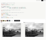 Halide box-7 code: A blur written as a reduction rather than as named taps, live: an RDom over the window, a pure definition that zeroes the accumulator, an update definition that accumulates the window. Figure 29.4.7: Chapter 29.4, Halide programming
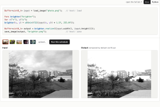 Halide brighten: one line of arithmetic on a real image, run in the page: multiply by 1.5 in floating point, clamp at 255, cast back to 8 bits. Figure 29.4.5: Chapter 29.4, Halide programming
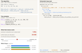 compute_at, and the loops it produces: the algorithm is fixed and the schedule is yours; change it and read the loop nest that comes out. Figure 29.4.11: Chapter 29.4, Halide programming
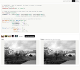 Halide first program: the running example as a complete program, live. Figure 29.4.1: Chapter 29.4, Halide programming
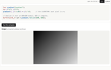 Halide gradient: the smallest complete Halide program, and its output. Figure 29.4.4: Chapter 29.4, Halide programming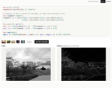
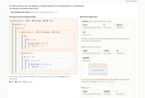 Halide granularity: where each producer is computed, and what that costs. Figure 29.4.12: Chapter 29.4, Halide programming
 Halide hist: the scatter reduction: the bin an update writes to is chosen by the pixel value, so Halide cannot simply vectorize or split the loop, and parallel execution must handle collisions between updates. Figure 29.4.8: Chapter 29.4, Halide programming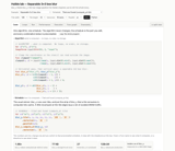
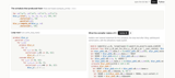 Halide loop nest: A schedule, and the loop nest Halide generates from it, side by side. Figure 29.4.9: Chapter 29.4, Halide programming
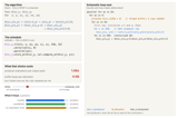 store_at against compute_at: the same two-stage blur with one dial added, where the producer's buffer lives, separately from where it is computed. Figure 29.5.1: Chapter 29.5, Scaling up Halide
 Halide bilateral-grid graph: the bilateral grid as a graph: gray splats into histogram , the 3-D grid; three blurs run along the grid's z, x and y axes; an interpolation stage slices the blurred grid back onto the image. Figure 29.5.12: Chapter 29.5, Scaling Up Halide
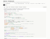 Halide bilateral-grid lab: the whole lab on the bilateral grid. Figure 29.5.14: Chapter 29.5, Scaling Up Halide
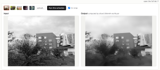 Halide bilateral-grid result: edge-preserving smoothing from the grid, run in the page: with cells eight pixels wide, texture is flattened well past what the 5×5 brute force reaches, with the approximation’s result visible alongside the input. Figure 29.5.13: Chapter 29.5, Scaling Up Halide
 Halide bilateral graph: the bilateral filter as a graph: gray feeds both num and den with a 5×5 footprint, and the two meet again at the divide. Figure 29.5.9: Chapter 29.5, Scaling Up Halide
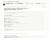 Halide bilateral lab: the whole lab on the bilateral filter. Figure 29.5.11: Chapter 29.5, Scaling Up Halide
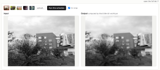 Halide bilateral result: edge-preserving smoothing, run live: texture and noise are flattened while the boundaries between regions stay sharp. Figure 29.5.10: Chapter 29.5, Scaling Up Halide
 Halide box-7 graph: the 7×7 box blur as a graph of stages: the clamped input feeds total , which accumulates 49 values per output pixel, and total feeds the divide. Figure 29.5.3: Chapter 29.5, Scaling Up Halide
 Halide box-7 lab: the whole lab on the reduction: switch the schedule between root, per-scanline and tiled, inspect the loop nest around the update definition and time each schedule. Figure 29.5.5: Chapter 29.5, Scaling Up Halide
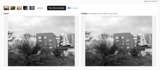 Halide box-7 result: what it does to a photograph: input and output side by side, zoomed into a crop so a 7-pixel-wide average is visible at page size, computed with the selected schedule. Figure 29.5.4: Chapter 29.5, Scaling Up Halide
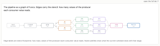 Halide harris graph: Harris as a graph: ten stages and fifteen edges between the input and the corner map, laid out in layers. Figure 29.5.6: Chapter 29.5, Scaling Up Halide
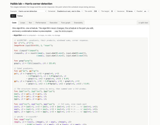 Halide harris lab: the whole lab on the corner detector. Figure 29.5.8: Chapter 29.5, Scaling Up Halide
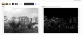 Halide harris result: the corner response, computed in the browser. Figure 29.5.7: Chapter 29.5, Scaling Up Halide
 Halide pyramid graph: the pyramid as a graph: two downsamples to build the Gaussian levels, upsamples and differences to get the detail bands, a multiply to boost them, and reconstruction from the modified bands. Figure 29.5.15: Chapter 29.5, Scaling Up Halide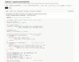
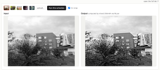 Halide pyramid result: local contrast enhancement from a Laplacian pyramid, computed live: the detail bands are amplified and added back, so texture comes forward while the coarse image content is retained. Figure 29.5.16: Chapter 29.5, Scaling Up Halide
45.26.12 Edges matter⧉
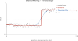 Bilateral 1-D: drag σ_s / σ_r on a noisy step edge; small σ_r keeps the edge. Figure 10.1.1: Chapter 10.1, Bilateral filtering
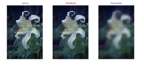 Bilateral on an image: the bilateral filter on a real photo, vs a plain Gaussian. Figure 10.1.4: Chapter 10.1, Bilateral filtering
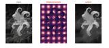 Bilateral kernels: the space-varying kernel made visible, patch by patch. Figure 10.1.5: Chapter 10.1, Bilateral filtering
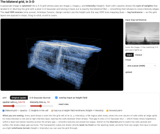 Bilateral grid (3-D): the 3-D bilateral grid: splat, blur, slice, orbitable. Figure 10.1.10: Chapter 10.1, Bilateral filtering
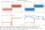 Bilateral grid (1-D): one scanline splatted into a position-intensity grid, blurred, sliced and divided, against brute force and a plain downsample. Figure 10.1.11: Chapter 10.1, Bilateral filtering
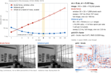 Bilateral speed: brute force against the grid: brute-force bilateral and bilateral grid as Halide wasm, timed in the reader's browser over σs = 1 to 32 px, with the crossover, the grid's bins in x, y and range, and both outputs. Figure 10.1.16: Chapter 10.1, Bilateral filtering
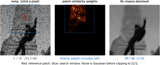 Non-local means: click a pixel and see which patches it averages, wherever they are. Figure 10.2.2: Chapter 10.2, Non-local means
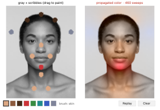 Colorization by scribbles: chrominance flooded from a few strokes, halting at luminance edges. Figure 10.3.1: Chapter 10.3, Edge-preserving optimization — colorization
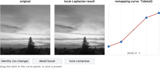 Local Laplacian filtering: an editable remapping curve for detail and tone control designed to reduce halos. Figure 10.4.8: Chapter 10.4, Local Laplacian filters
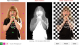 Closed-form matting: pull a soft matte from a few strokes via the matting Laplacian. Figure 10.5.5: Chapter 10.5, Matting Laplacian
 Poisson blending: seamless cloning in linear/gamma/log spaces, with mixed gradients. Figure 10.8.5: Chapter 10.8, Poisson image editing
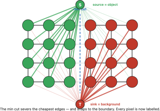 Graph-cut construction: the min-cut network built up step by step on a toy grid. Figure 10.9.2: Chapter 10.9, Seam optimization
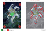 Graph-cut segmentation (live): scribble object/background seeds; a max-flow finds the exact cut. Figure 10.9.3: Chapter 10.9, Seam optimization
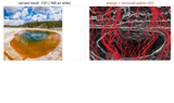 Seam carving: content-aware resize by dynamic-programming seams, traced live. Figure 10.9.5: Chapter 10.9, Seam optimization
45.26.13 Warping and morphing⧉
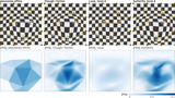 Smooth triangulation warps: one set of controls warped piecewise affinely, by Clough–Tocher and by Loop and butterfly subdivision, with Loop's misses, the solve that removes them, and Loop-subdivided blending weights. Figure 11.1.7: Chapter 11.1, Warping
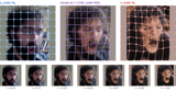 Two-pass mesh warp: Smythe's spline grid warp for Willow, pass by pass, against triangles and bilinear cells, and the mesh morph. Figure 11.1.8: Chapter 11.1, Warping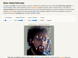
 Liquify demo: interactive Liquify, a mesh warp driven by a brush. Figure 11.1.12: Chapter 11.1, Warping
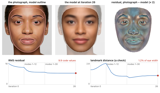 2-D morphable face model: a face model learned from 951 photographs, shown at every step (correspondence, Procrustes, modes, face space, shape and appearance, a pixel fit by analysis by synthesis), with sliders, random faces and morphs. Figure 11.4.1: Chapter 11.4, Morphable models
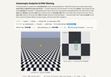 EWA / anisotropic footprint: nearest/bilinear/MIP/EWA on a receding floor, with the footprint ellipse. Figure 11.2.6: Chapter 11.2, Antialiasing for complex transforms
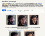 Beier–Neely morph: a two-image feature morph with cross-dissolve. Figure 11.3.4: Chapter 11.3, Morphing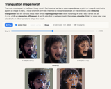
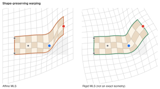 Shape-preserving warp: naive affine MLS (shears) vs rigid/similarity MLS (bends). Figure 11.5.2: Chapter 11.5, Shape-preserving warping
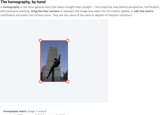
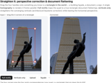 Perspective rectify: drag four corners to fronto-parallel a page/façade. Figure 11.6.3: Chapter 11.6, Perspective distortion and its correction
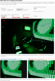 Wide angle crop: cropping a wide-angle photo, two ways. Figure 11.6.6: Chapter 11.6, Perspective distortion and its correction
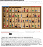 Perspective montage: head-on shots vs a single-camera unified scene, with a focal-length slider. Figure 11.6.13: Chapter 11.6, Perspective distortion and its correction
45.26.14 Matching pixels across space and time⧉
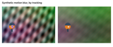 Track → motion blur: track a point, stabilize, average, motion-blur. Figure 12.4.5: Chapter 12.4, Feature tracking
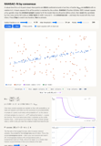 RANSAC: robust fitting, step by step. Figure 12.5.3: Chapter 12.5, Robustness: the ratio test and RANSAC
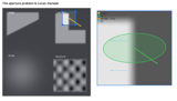 Aperture problem & Lucas–Kanade: why local flow is ambiguous, and when a Lucas–Kanade neighborhood supplies enough constraints. Figure 12.8.5: Chapter 12.8, Optical flow
 Live face landmarks: MediaPipe 478-point face mesh with mesh/makeup/hat overlays. Figure 12.10.2: Chapter 12.10, Face tracking
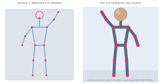 Pose puppet: MediaPipe BlazePose skeleton over your camera feed or a photo. Figure 12.11.2: Chapter 12.11, Body pose estimation
45.26.15 Single-image computational photography⧉
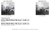 BM3D: group / collaborative-filter / aggregate, made visible. Figure 13.6.3: Chapter 13.6, Non-local means and BM3D
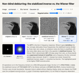 Wiener deconvolution: naive inverse filter (explodes) vs Wiener, with MTF and PSNR. Figure 16.2.2: Chapter 16.2, Non-blind deconvolution
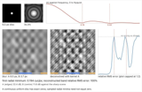 Defocus zeros: grow a defocus disc and watch the zeros of its transfer function move inward, then deconvolve two depths with one kernel. Figure 16.6.1: Chapter 16.6, Defocus and undoing what the lens softened
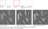 Kernel error ratio: four classical kernel estimators on one blur, scored by the error ratio rather than by how convincing the result looks. Figure 16.9.1: Chapter 16.9, Measuring a deblur
 Shannon n-grams: an order-n Markov model congealing gibberish into English (the ancestor of texture synthesis). Figure 21.1.6: Chapter 21.1, Inpainting, texture synthesis, and object removal
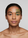 Clone vs heal brush: clone copies pixels; heal copies texture but adopts local tone. Figure 21.1.12: Chapter 21.1, Inpainting, texture synthesis, and object removal
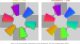 Premultiplied alpha: why RGBA must be filtered premultiplied, or edges get a dark fringe. Figure 19.1.1: Compositing, segmentation and matting
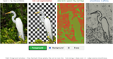 Graph-cut segmentation (min-cut): contrast-sensitive t-links/n-links partition foreground from background. Figure 19.2.2: Compositing, segmentation and matting
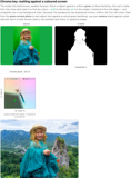 Chroma key: green/blue-screen matting, camera-capable. Figure 19.3.1: Compositing, segmentation and matting
45.26.16 Compound lenses and aberration correction⧉
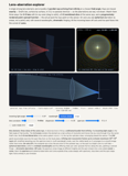 Aberration explorer: A single strong lens element and a bundle of parallel rays arriving from infinity at a chosen field angle, traced exactly by Snell's law. Figure 22.1.6: Chapter 22.1, Aberrations and optical challenges
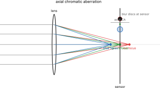 Axial chromatic aberration: R/G/B focus at different depths. Figure 22.1.8: Chapter 22.1, Aberrations and optical challenges
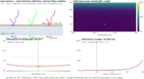 Coating reflectance: anti-reflection coatings, over wavelength and angle. Figure 22.1.15: Chapter 22.1, Aberrations and optical challenges
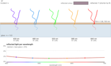 Coating thin film: an anti-reflection coating, wave by wave. Figure 22.1.16: Chapter 22.1, Aberrations and optical challenges
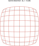 Barrel ↔ pincushion: dial radial distortion on a ruled grid. Figure 22.1.10: Chapter 22.1, Aberrations and optical challenges
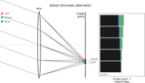 Lateral chromatic aberration: R/G/B magnified differently, fringes toward the frame edge. Figure 22.1.9: Chapter 22.1, Aberrations and optical challenges
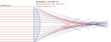 Paraxial vs Snell: real Snell rays vs the thin-lens model; the gap is spherical aberration. Figure 22.1.3: Chapter 22.1, Aberrations and optical challenges
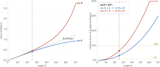 Small-angle approximation: how far sin θ ≈ θ holds; the error is cubic. Figure 22.1.1: Chapter 22.1, Aberrations and optical challenges
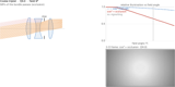 Vignetting: vignetting, ray-traced on the usual Cooke triplet. Figure 22.1.12: Chapter 22.1, Aberrations and optical challenges
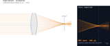 Aspheric elements: one aspheric surface versus a stack of spheres. Figure 22.2.4: Chapter 22.2, Aberrations correction
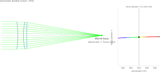 Achromat / hybrid correction: real ray tracing showing how a doublet or diffractive surface reduces chromatic aberration. Figure 22.2.3: Chapter 22.2, Aberrations correction
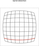 Radial distortion correction: drag k1/k2 to bow a grid, then toggle the cure. Figure 22.2.7: Chapter 22.2, Aberrations correction
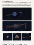 Lens optimizer: a multi-element lens optimized by damped least squares over fields and wavelengths. Figure 22.4.4: Chapter 22.4, Lens optimization
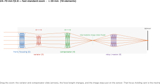 Modern zoom designs: inside a complex modern zoom. Figure 22.5.5: Chapter 22.5, A short bestiary of classic designs
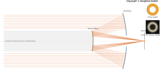 Catadioptric mirror lens: the catadioptric (mirror) telephoto, ray-traced. Figure 22.7.5: Chapter 22.7, Special optics
- A defocus-control lens: the Nikon 135 mm f/2 DC and its second ring, which adjusts spherical aberration and can require refocusing. Figure 22.7.11: Chapter 22.7, Special optics
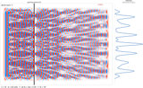 Diffraction grating: a live 2-D wave breaking into orders; change λ and watch them sweep. Figure 22.7.15: Chapter 22.7, Special optics
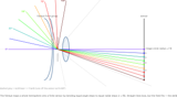 Fisheye ray-trace: A fisheye lens in cross-section, ray-traced. Figure 22.7.4: Chapter 22.7, Special optics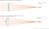
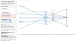
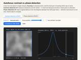 Autofocus: contrast-detection (hill-climb) vs phase-detection (estimated direction and amount of defocus). Figure 22.9.3: Chapter 22.9, Autofocus
 Acuity chart: visual acuity, read off an eye chart. Figure 22.12.4: Chapter 22.12, The eye as an optical instrument: vision and its correction
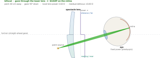 Bifocal eye ray-trace: presbyopia corrections in front of the eye, ray-traced. Figure 22.12.8: Chapter 22.12, The eye as an optical instrument: vision and its correction
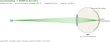 Eye accommodation: the eye as an autofocusing camera, ray-traced. Figure 22.12.2: Chapter 22.12, The eye as an optical instrument: vision and its correction
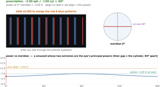 NETRA refraction: A phone as a phoropter: the NETRA alignment game. Figure 22.12.6: Chapter 22.12, The eye as an optical instrument: vision and its correction
 Refractive errors: the eye out of focus, and the spectacle lens that fixes it. Figure 22.12.3: Chapter 22.12, The eye as an optical instrument: vision and its correction
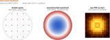 Shack–Hartmann sensor: measuring the eye's wavefront: the Shack-Hartmann sensor. Figure 22.12.5: Chapter 22.12, The eye as an optical instrument: vision and its correction
45.26.17 Multiple-exposure imaging⧉
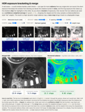
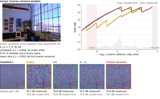 Optimal HDR merge weights: merge a simulated bracket with binary, hat, k_i-proportional and inverse-variance weights and compare the merged SNR against radiance, measured and in closed form. Figure 17.3.4: Chapter 17.3, Merging exposures
 Full HDR pipeline: MTB align → Debevec response recovery → merge → tone-map. Figure 17.2.3: HDR merging
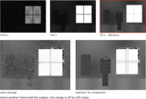 HDR ghosting: merge brackets of a moving subject four ways and see how much of the ghost precision weighting removes before any rejection. Figure 17.4.3: Chapter 17.4, Ghosts and motion
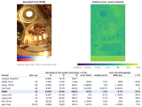 HDR formats, round trip: one radiance map through eight HDR formats and back, with a per-pixel error map, a probe table and bits per pixel. Figure 17.7.4: Chapter 17.7, Encoding HDR images
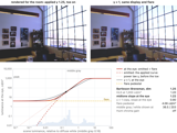 System gamma simulator: a radiance map rendered for a surround, a display peak and a flare level, with the end-to-end curve and its measured midtone slope. Figure 18.1.1: Chapter 18.1, Tone mapping and perception
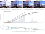 Four global operators compared: Ward, Drago, Reinhard and histogram adjustment on one radiance map, with each curve and its contrast gain G. Figure 18.2.2: Chapter 18.2, Global tone mapping
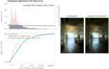 Histogram adjustment, step by step: Ward Larson's histogram adjustment on a radiance map in stages, from the log histogram and its equalization curve to the slope ceiling, trimming pass by pass and the final curve, with a Weber or threshold-versus-intensity ceiling. Figure 18.2.8: Chapter 18.2, Global tone mapping
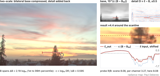 From a global curve to two-scale tone mapping: one radiance map compressed per channel, on the luminance with color ratios kept, then with a Gaussian and a bilateral base, with a probe, base and detail layers, and a profile across a strong edge. Figure 18.3.1: Chapter 18.3, Two-scale and bilateral tone mapping
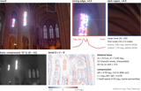 Two-scale explorer: one radiance map split into base and detail by a Gaussian, bilateral, WLS or guided base, with magnifiers on a strong edge and a dark region. Figure 18.3.6: Chapter 18.3, Two-scale and bilateral tone mapping
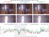 Multiscale tone mappers at matched compression: per-band gains, subband companding and the local Laplacian filter on one radiance map, with a magnifier and a scanline across a strong edge. Figure 18.5.1: Chapter 18.5, Local Laplacian filtering and other multiscale methods
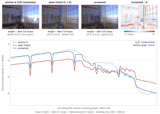 Screened gradient-domain tone mapping: Fattal's gradients anchored to a low-resolution two-scale map, with the crossover scale on a slider. Figure 18.6.3: Chapter 18.6, Gradient-domain tone mapping
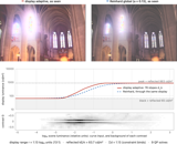 Display-adaptive tone mapping: the tone curve solved for a display's peak, black level and ambient light, against Reinhard's. Figure 18.7.1: Chapter 18.7, Tone mapping as perceptual optimization
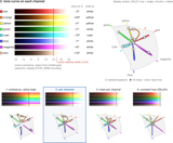 Hue paths through view transforms: eight saturated colors ramped through four view transforms that share one tone curve, with their hue and chroma paths. Figure 18.8.2: Chapter 18.8, Display rendering transforms and color
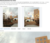 Manual panorama: four point-pairs → reproject and blend. Figure 20.1.5: Chapter 20.1, Manual panorama stitching from multiple views
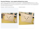 Document flatten: drag four corners of a page to a fronto-parallel scan. Figure 20.1.6: Chapter 20.1, Manual panorama stitching from multiple views
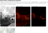 Harris corners: the Harris detector, component by component. Figure 20.2.2: Chapter 20.2, Automatic panorama stitching from multiple views and feature matching
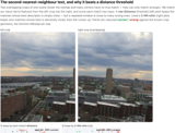 Second-nearest-neighbor test: the value of the ratio test for feature matching. Figure 20.2.3: Chapter 20.2, Automatic panorama stitching from multiple views and feature matching
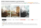 RANSAC (panorama): robust homography estimation, step by step. Figure 20.2.5: Chapter 20.2, Automatic panorama stitching from multiple views and feature matching
 Multiband blending: hard cut / feather / 2-scale / full Laplacian-pyramid blend, per-band. Figure 20.3.4: Chapter 20.3, Blending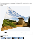
 Panorama viewer: a 360° equirectangular panorama on a sphere, viewed from inside. Figure 20.4.5: Chapter 20.4, Bells and whistles
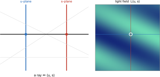 Two-plane (u, s) parametrization: name a ray by where it crosses two planes; sub-aperture views and points. Figure 23.3.7: Chapter 23.3, Focal stacks and depth of field extension
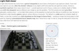 Light-field viewer: shift-and-add refocus, synthetic aperture, and parallax over a real capture. Figure 23.3.8: Chapter 23.3, Focal stacks and depth of field extension
45.26.18 Many images and photo collections⧉
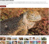 Photomosaic: hover to magnify a photomosaic so the tile photos become legible. Figure 28.1.1: Chapter 28.1, Photo Mosaics
 CLIP-IQA curation: a real CLIP model scores and ranks a photo set for quality in-browser. Figure 28.3.2: Chapter 28.3, Auto curation
 Photobio time-lapse: aligned portraits picked and cross-faded into an aging time-lapse. Figure 28.6.2: Chapter 28.6, Photobios
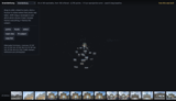 Photo tourism explorer: fly through a landmark reconstructed from strangers' photographs, click a camera frustum to enter that photograph, and drag a box over a detail to be taken to the view that shows it best. Figure 28.5.4: Chapter 28.5, Photo tourism
 KD-tree collage: a canvas recursively bisected so every photo gets its own cell. Figure 28.12.2: Chapter 28.12, Displaying images together
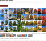 SOM collage: a self-organizing-map layout where similar photos sit as neighbors. Figure 28.12.4: Chapter 28.12, Displaying images together
45.26.19 Video⧉
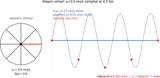 Wagon-wheel effect: temporal aliasing: a spoked wheel stalls or reverses above Nyquist. Figure 30.1.6: Chapter 30.1, Motion blur, temporal sampling, and resampling
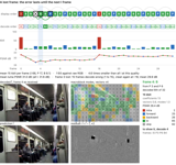 I, P and B frames: a small MPEG-style codec on real video: GOP, decode order, bits and PSNR per frame, seeking, and drift after a lost frame. Figure 30.2.1: Chapter 30.2, Video compression and motion compensation
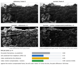 Temporal redundancy on real video: plain frame difference against motion-compensated residual on four real clips, with measured bits per pixel for still, difference and motion-compensated coding; add a camera pan or zoom. Figure 30.2.2: Chapter 30.2, Video compression and motion compensation
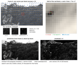 Block-matching motion search: block motion vectors on real video, a clicked block's SAD surface, full against three-step and diamond search, whole against half pixel, with the prediction and its residual. Figure 30.2.3: Chapter 30.2, Video compression and motion compensation
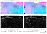 Dense flow against block vectors: Horn–Schunck optical flow beside a codec's block vectors on the same frames, each residual and the bits of residual plus field. Figure 30.2.5: Chapter 30.2, Video compression and motion compensation
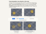 Frame interpolation: flow-based interpolation vs a naive cross-dissolve. Figure 30.4.4: Chapter 30.4, Frame interpolation and slow-motion synthesis
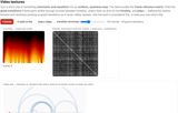 Video textures: build the frame-distance matrix, find transitions, play an endless loop. Figure 30.8.2: Chapter 30.8, Video textures
45.26.20 Light fields and plenoptic cameras⧉
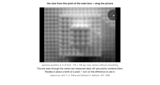 Adelson and Wang's own capture: a 1992 plenoptic capture of a Lego pyramid; drag the picture to move your viewpoint around the lens aperture. Figure 31.2.4: Chapter 31.2, Light field cameras
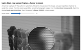 Lytro raw loupe: hover-zoom a real Lytro Illum raw frame: honeycomb → sub-aperture discs → Bayer. Figure 31.2.13: Chapter 31.2, Light field cameras
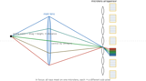 Plenoptic camera: how a plenoptic camera maps rays to sub-pixels, in scene and aperture modes. Figure 31.2.7: Chapter 31.2, Light field cameras
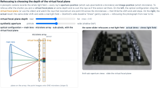 Refocus shift geometry: the optical configuration and a real captured light field refocused by one slider. Figure 31.4.2: Chapter 31.4, Refocusing and synthetic aperture
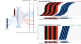 LF aberration interactive: try it yourself (web edition). Figure 31.5.2: Chapter 31.5, Aberration correction in light fields
45.26.21 Computational illumination⧉
- Edgerton's high-speed classics: the Milk Drop Coronet and a Rapatronic fireball, the two exposures that defined stroboscopic photography. Figure 35.2.2: Chapter 35.2, High-speed and stroboscopic photography
45.26.22 3-D and depth⧉
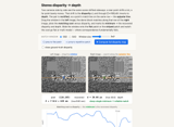
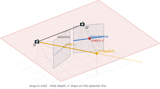 Epipolar line: a pixel back-projects to a ray that images as a line in the other view. Figure 36.1.6: Chapter 36.1, Multiple view geometry
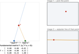 Fundamental matrix: epipolar geometry with F computed live from two cameras. Figure 36.1.8: Chapter 36.1, Multiple view geometry
 Gaussian splat viewer: an interactive 3-D Gaussian-splatting scene: drag to orbit, scroll to zoom. Figure 36.7.7: Chapter 36.7, Photos → radiance fields and Gaussian splatting (NeRF, 3DGS)
45.26.23 Revealing the invisible⧉
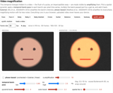 Video magnification demo: try it yourself. Figure 38.3.7: Chapter 38.3, Motion and video magnification
45.26.24 Appendices and end matter⧉
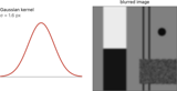 Gaussian blur: drag σ and watch a separable Gaussian blur a synthetic test image. Figure 45.2.7: Chapter 45.2, Refreshers
 Museum of Computational Photography: the animated 3-D cover. Figure 45.18.1: Chapter 45.18, How this book was created (the early process)
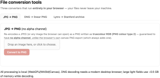 File conversion tools: three browser-only converters (JPG→PNG no-alpha, DNG→linear PNG, Lytro→Stanford archive). Figure 45.24.1: Chapter 45.24, File conversion tools
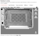 Photoshop 1.0: Adobe Photoshop 1.0 (1990) running on an emulated Macintosh II; boot it, let the page drive the mouse to launch it, and run the 1990 filters on one of this book's photographs. Figure 45.33.1: Chapter 45.33, Photoshop 1.0, running
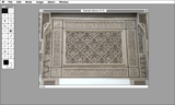 Photoshop 1.0 in JavaScript: Adobe Photoshop 1.0 rebuilt as a web application, menus, dialogs and tools reproduced from the source's resource fork, running the transcribed 1990 arithmetic. Figure 45.34.1: Chapter 45.34, Photoshop 1.0 ported to JavaScript
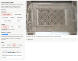 The 1990 filters: Photoshop 1.0.1's own routines, transcribed out of Adobe's source and run on a modern photograph: Gaussian Blur, Unsharp Mask, Find Edges, Median, Despeckle, Sharpen Edges and the Custom 5 by 5, with a readout of what each one is doing inside. Figure 45.34.2: Chapter 45.34, Photoshop 1.0 ported to JavaScript
45.26.25 Not yet placed⧉
A few interactive modules live in the figure library but are not yet referenced in a drafted chapter. They are listed here for completeness and will fold into the index above once their chapters are written or their host is finalised:
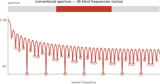 the figure: a coded aperture keeps a broadband spectrum (no deep zeros), so the blur is invertible; destined for the coded-imaging part.
 the figure: the parent collage viewer, split in the book into the photomosaic, KD-tree and SOM demos above.
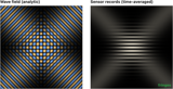 Figure 2.1.11: built in the figure library, not yet placed in a drafted chapter.
 the figure: wavelet-coring denoisers scored by PSNR against the clean original; written for the denoising chapter, not yet placed in it.
 the figure: a gallery of flash from magnesium powder to the modern speedlight; built in the figure library, not yet placed in a drafted chapter.
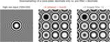 the figure: decimating a zone plate with vs without a Gaussian prefilter (a sampling demo).
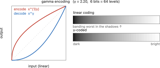 the figure and the figure: gamma coding on a ramp and on a photo; superseded in the book by the combined gamma + quantization banding demo above.
 the figure: built in the figure library, not yet placed in a drafted chapter.
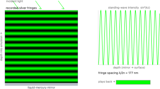 the figure: built in the figure library, not yet placed in a drafted chapter.
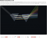 the figure: built in the figure library, not yet placed in a drafted chapter.
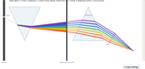 the figure: built in the figure library, not yet placed in a drafted chapter.
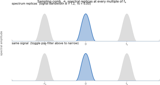 the figure: sampling as multiplication by a Dirac comb; listed in the Part 6, Linear methods and Fourier analysis outline, its chapter not yet drafted.
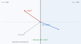 the figure: Snell's law traced ray by ray; superseded by the combined reflection / refraction / diffraction demo above.
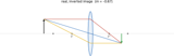 the figure: the three principal rays locating an image; companion to the thin-lens conjugates demo above.