15.4 Optimizing and searching classical demosaickers⧉
The demosaickers of Chapter 15.1, Basic traditional demosaicking and Chapter 15.2, Advanced traditional demosaicking were designed by hand, and so were their numbers: the quarter and half weights of Hamilton–Adams, the gains of Malvar–He–Cutler, the threshold of VNG, the window and regularization of a guided filter. Between that and a fully learned network (Chapter 15.6, Learned demosaicking) lies a middle ground that this chapter is about. Keep the structure of a classical method, which is small, fast and understandable, and let data decide either its parameters, by gradient descent, or its structure itself, by search. The result can still run on a camera's image signal processor, which is where hand-designed methods still dominate, and it can be tuned to a particular sensor, noise level or cost budget in a way no hand-tuning would.
15.4.1 Fitting a classical demosaicker by gradient descent⧉
A classical demosaicker is a short program made of linear filters, a few nonlinear decisions and some arithmetic, and most of its constants are continuous. If the program is differentiable with respect to those constants, they can be fitted like the weights of a network: take full-color images, mosaic them, run the demosaicker, compare its output with the originals, and descend the gradient of the error (Chapter 15.11, Synthetic data, unprocessing, and raw reconstruction discusses where such pairs come from and what they cost in realism).
Two things stand in the way, and both have standard answers.
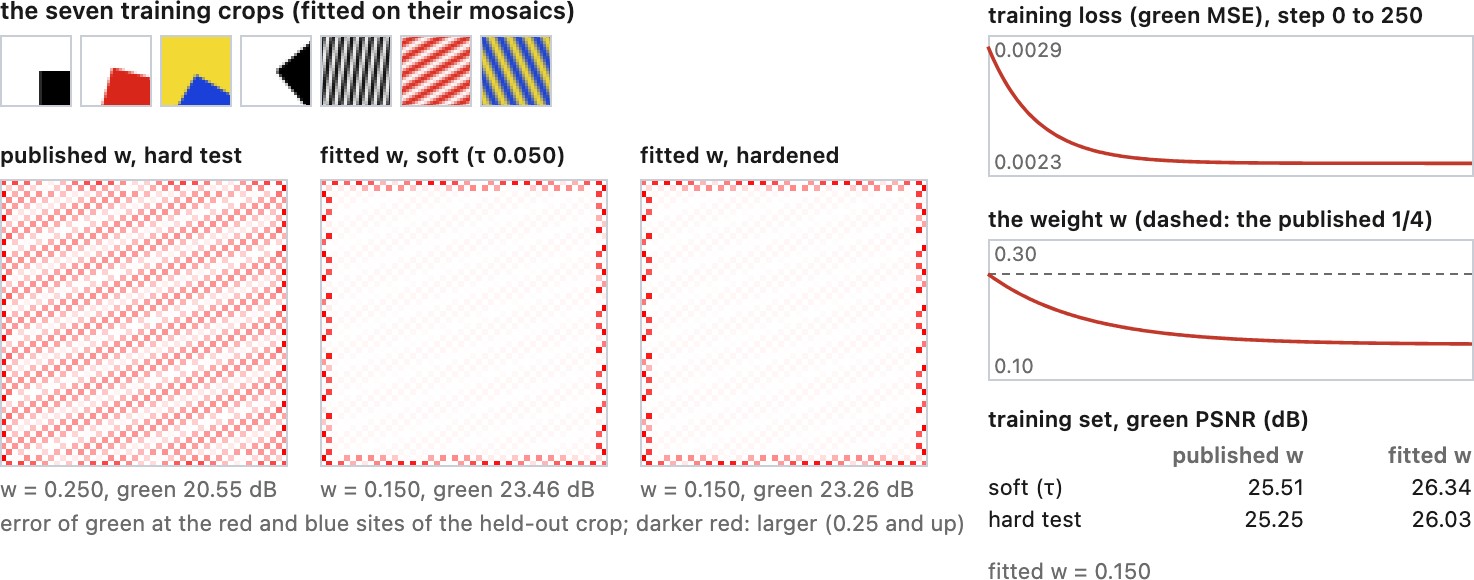
Hard decisions. A direction test, "interpolate horizontally if $d_H<d_V$", has no useful derivative: an infinitesimal change of the parameters either leaves the choice alone or flips it. The usual fix is to replace the hard choice by a soft one during training, blending the two directional estimates with weights that depend smoothly on the two costs, for example $w_H = e^{-d_H/\tau}/(e^{-d_H/\tau}+e^{-d_V/\tau})$. The temperature $\tau$ controls how hard the blend is; lowering it during training and hardening the choice at deployment recovers a program that makes the same decisions as the original, with fitted constants.
Computing the derivative efficiently. Automatic differentiation in a deep-learning framework works but is slow for pipelines written as many small stencils. Gradient Halide Li et al. 2018 generates the derivative of a Halide image-processing pipeline automatically and schedules it like any other pipeline, so the same algorithm description is trained efficiently and then compiled for the device (Gradient Halide: differentiating the pipeline).
# Fit the constants of a soft Hamilton-Adams green step on training pairs
params = {"w_corr": 0.25, "tau": 1.0}                    # start from the published values
for step in range(num_steps):
    mosaic, target = sample_training_pair()               # full-color image and its mosaic
    dH = abs(Gl - Gr) + abs(2*C - Cl2 - Cr2)              # gradients from the mosaic
    dV = abs(Gu - Gd) + abs(2*C - Cu2 - Cd2)
    gH = (Gl + Gr)/2 + params["w_corr"] * (2*C - Cl2 - Cr2)
    gV = (Gu + Gd)/2 + params["w_corr"] * (2*C - Cu2 - Cd2)
    wH = softmax([-dH, -dV] / params["tau"])[0]           # soft choice during training
    G  = wH * gH + (1 - wH) * gV
    loss = mean((G - target_green)**2)
    params -= lr * gradient(loss, params)
    params["tau"] *= anneal                               # harden the choice over time
# deploy with the hard test and the fitted w_corr
Figure 15.4.1 runs this loop on the correction weight.
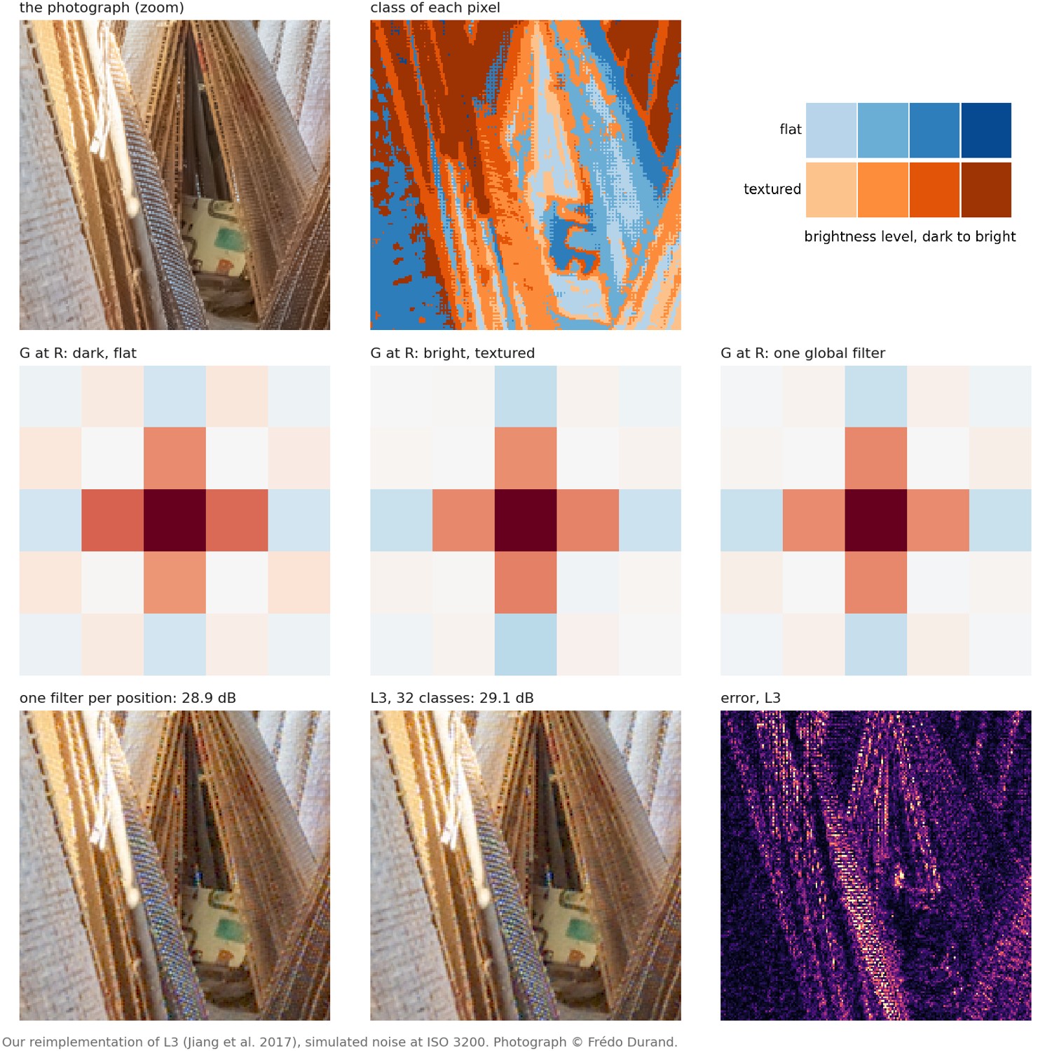
The same idea predates automatic differentiation wherever the parameters enter linearly. Malvar, He and Cutler derived the gains of their filters from a Wiener-filter fit to a standard set of test images Malvar et al. 2004, and Leung, Jeon and Dubois designed the filters of frequency-domain demosaicking by least squares (Chapter 15.2, Advanced traditional demosaicking, Leung, Jeon & Dubois 2011 (least-squares luma-chroma demultiplexing)). The L3 approach, local, linear and learned, of Jiang and colleagues Jiang et al. 2017 (L3) classifies each pixel by a few local features, such as its color channel, its brightness and how much texture surrounds it, and applies a linear filter learned by least squares for that class: a table of small classical filters chosen by a classical test, with every filter fitted to data. RAISR does the same for upsampling (Chapter 14.4, Single-image super-resolution: classical methods).
On one photograph at ISO 3200 (Figure 15.4.2), 32 classes improve on one filter per color position by a fraction of a decibel, and the learned filters differ where they should: in dark, flat regions, where noise dominates, the filter leans less on the pixel itself and averages more.
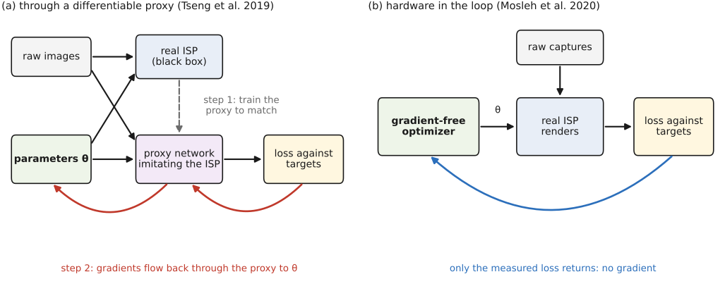
A camera's own image signal processor is the harder case, because its code is usually not available and not differentiable. Its parameters, dozens of them for demosaicking, denoising, sharpening and color, are still tuned by hand for each new sensor. Tseng and colleagues Tseng et al. 2019 (differentiable proxies) train a neural network to imitate the processor, a differentiable proxy, and optimize the parameters through the proxy's gradients; Mosleh and colleagues Mosleh et al. 2020 (hardware in the loop) instead optimize with the real hardware in the loop, using a search that needs only measured outputs. Both tune the classical pipeline's knobs rather than replacing it (Figure 15.4.3).
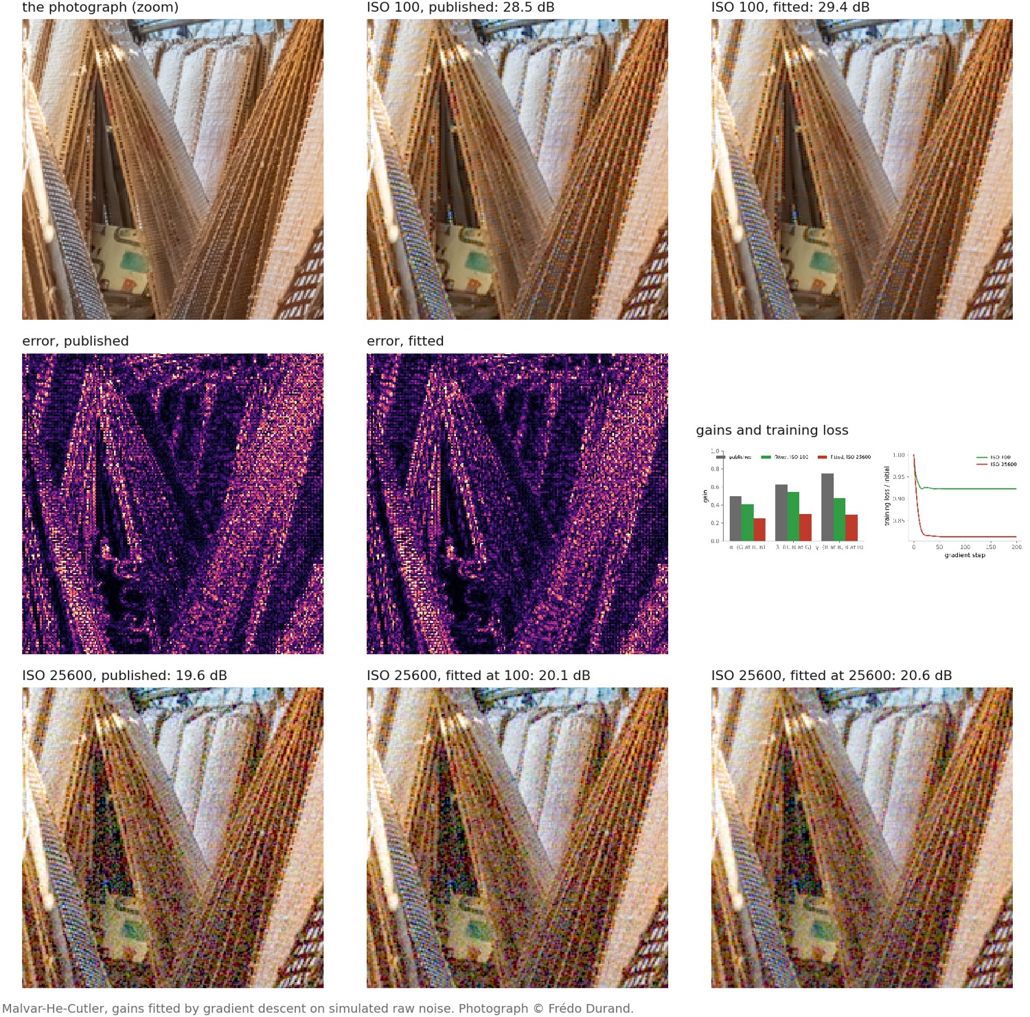
Fitting keeps what makes a classical method attractive: the program is as fast as before, its behavior can be read, and its failures are those of its structure. It also keeps that structure's limits. No choice of constants lets a two-direction test handle diagonal texture, and constants fitted to one sensor or noise level are no longer the best for another, so the evaluation data must match where the program will run.
Figure 15.4.4 shows the gain and its limit on Malvar, He and Cutler's three gains. Fitted at ISO 100, they come out smaller than the published ones and score about 0.9 dB better on a photograph that was not used for fitting. At ISO 25600 those gains still beat the published ones, but they are no longer the best: gains fitted at that ISO are about half as large, because each correction term is a Laplacian of a noisy channel and amplifies the noise.
15.4.2 Searching for the program itself⧉
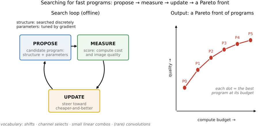
Gradient descent can tune the constants of a structure but cannot change the structure: there is no derivative of "add a second correction term" or "interpolate this difference instead of that one". Search can. Ma and colleagues' Searching for Fast Demosaicking Algorithms Ma et al. 2022 searches over demosaicking programs built from operations suited to the task, such as packing the mosaic's phases, small local linear combinations and separate reconstruction of green and of chroma, alongside conventional learned operations. A genetic search mutates the structure of candidate programs, gradient descent fits the constants of each candidate, and each is scored on two objectives, reconstruction quality and computational cost. The output is not one program but a family, one per budget, along a speed–quality Pareto front (Figure 29.8.2). The paper reports searched programs that trade cost for quality better than both classical methods and shrunk networks over the range it explores; the same framework produced programs for X-Trans mosaics and for joint demosaicking and super-resolution.
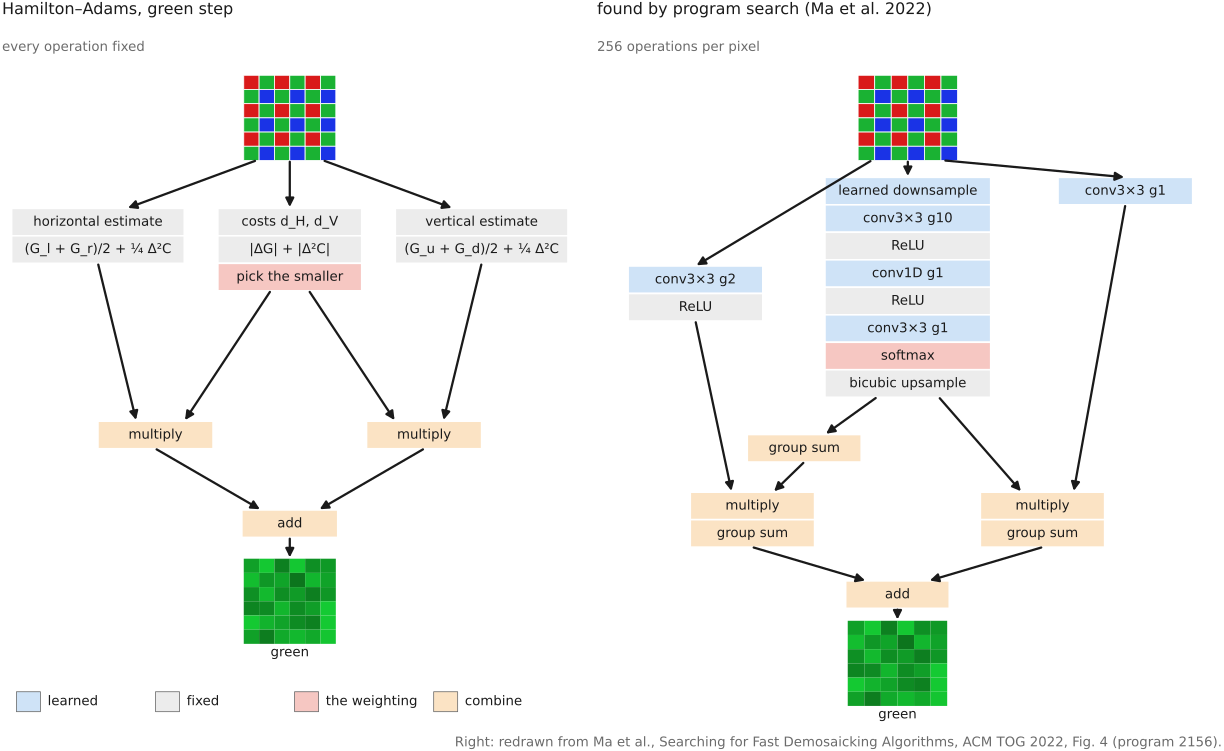
Drawn the same way, one of the programs the search found looks like a relative of Hamilton–Adams (Figure 15.4.5).
# program search in outline (see the code-speed part for the full protocol)
population = [classical_seed_programs()]                  # e.g. bilinear, Hamilton-Adams-like
for generation in range(G):
    children = [mutate(p) for p in select(population)]    # add, remove or rewire operations
    for p in children:
        fit_constants_by_gradient(p, training_pairs)       # the previous section, inside the search
        p.quality, p.cost = evaluate(p), operation_count(p)
    population = pareto_front(population + children)       # keep the non-dominated programs
compile_and_time(population)                               # measure on the real device
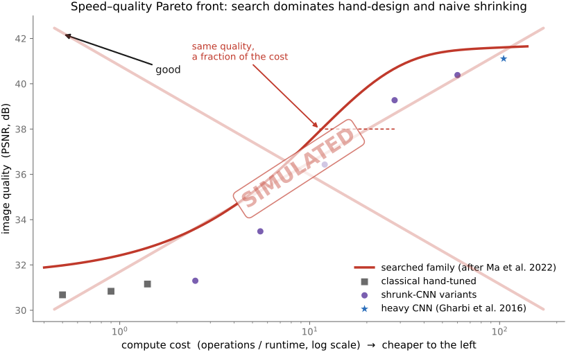
Searching programs has a history outside demosaicking. Sitthi-amorn and colleagues used genetic programming to simplify shaders, trading rendering error against speed in the same way Sitthi-amorn et al. 2011 (genetic shader simplification). And search can target the implementation rather than the algorithm: Halide's autoschedulers search how a fixed algorithm is executed, not what it computes. The two compose, and Chapter 29.8, Automatic search for fast methods treats both, with the evaluation protocol that keeps a search honest: separate data for fitting, for choosing among candidates and for the final test, and timing on the device rather than trusting an operation count.
What search gives the demosaicking problem is a way to reach the region the introduction to this part described, programs small enough for a camera's processor that are nonetheless shaped by data. What it does not give is a guarantee: the front is the best among the programs explored, in the chosen space of operations, for the chosen data and cost model.