fig-single-element-limit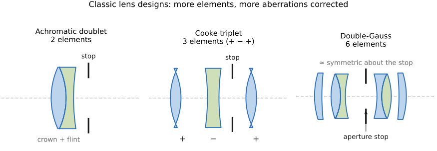
fig-doublet-triplet-gauss · cross-sections of three classic designs as stacked glass elements — achromatic doublet (2), Cooke triplet (3, + − +), double-Gauss (6, ≈symmetric about the stop); each labels element count and the aperture stop ✅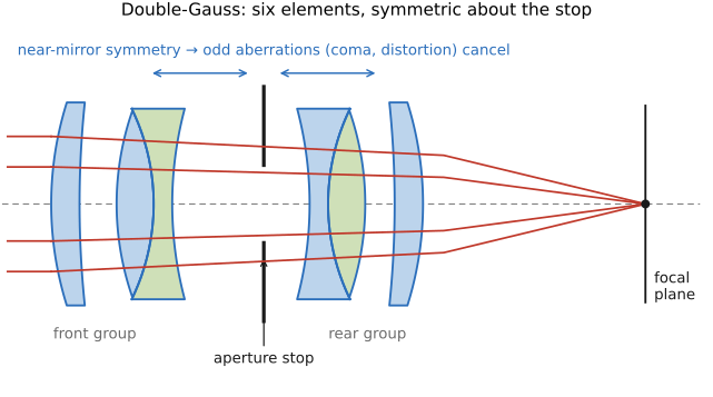
fig-double-gauss · a labeled double-Gauss cross-section: 6 elements ≈symmetric about the central aperture stop, parallel ray bundle traced to the focal plane; notes near-mirror symmetry cancels odd aberrations (coma, distortion, lateral color) ✅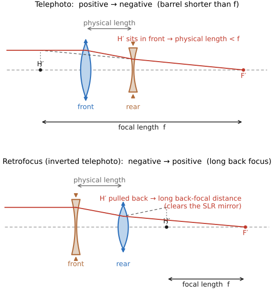
fig-telephoto-vs-retrofocus · two two-group schematics — telephoto (+ then −, principal plane H′ pushed in front → physical length < f) vs retrofocus/inverted-telephoto (− then +, long back-focal distance to clear the SLR mirror); marks f vs physical length, H′, F′ ✅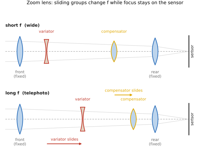
fig-zoom-mechanism · a zoom at two focal lengths (short-f/wide vs long-f/tele): moving variator + compensator groups slide along the axis to change f while the focal plane (sensor) stays fixed; motion arrows between states ✅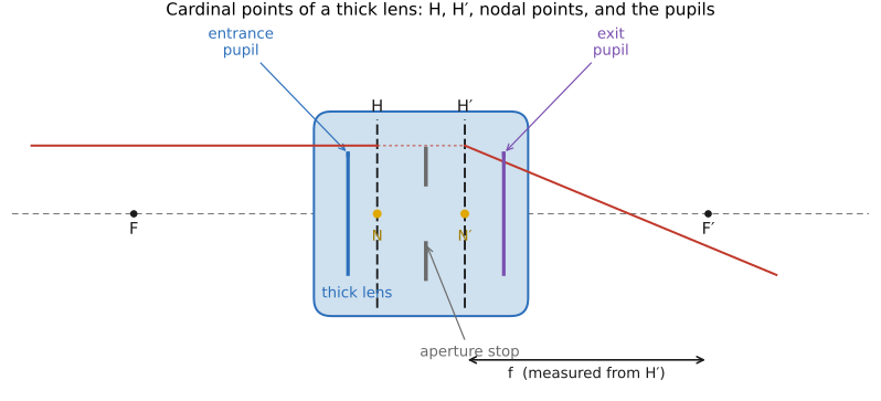
fig-principal-planes-pupils · a thick-lens cardinal-points diagram: principal planes H, H′, nodal points N, N′, entrance & exit pupils (the stop imaged by front/rear groups), focal points F, F′; f measured from H′ via the H→H′ equivalent-thin-lens construction ✅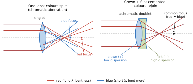
fig-achromat-doublet · an achromatic doublet: positive crown cemented to negative flint; singlet panel (red & blue split = chromatic aberration) vs doublet panel (red = blue at a common focus); labels crown/flint, low/high dispersion ✅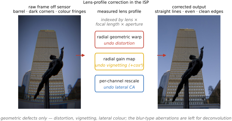
fig-lens-profile-correction · computational lens correction: a real window-grid facade degraded (barrel + vignette + lateral CA) → a measured profile's three radial maps (warp / gain / per-channel rescale) → corrected; note: geometric defects only, not blur (Aberrations correction) ✅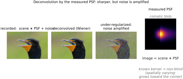
fig-psf-deconvolution · non-blind deconvolution by the measured PSF: a real crop convolved with a comatic PSF (inset) + noise → Wiener deconvolution (sharper) → under-regularized (noise amplified); image = scene ∗ PSF (Aberrations correction) ✅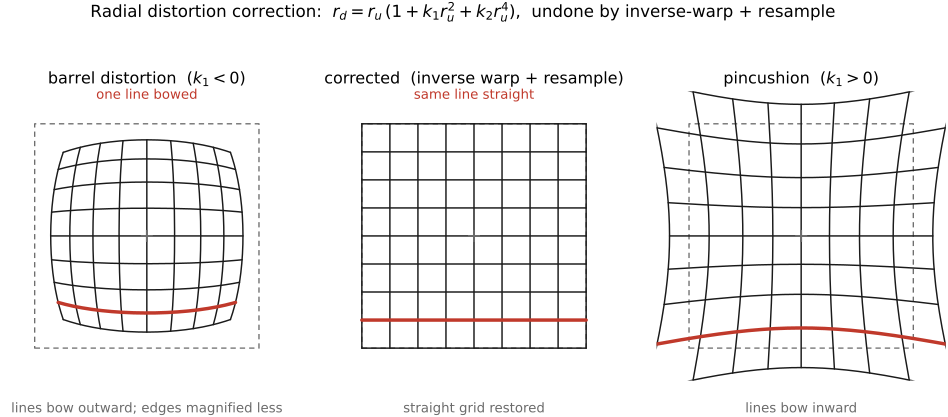
fig-radial-distortion-correction · 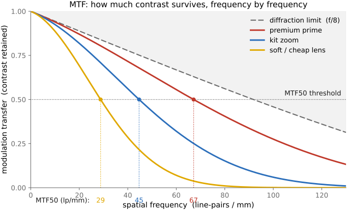
fig-mtf-curves · 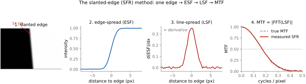
fig-slanted-edge-sfr · 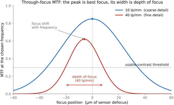
fig-mtf-through-focus · 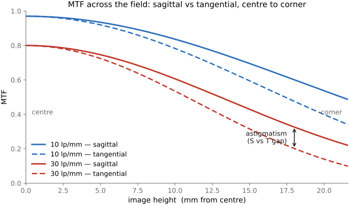
fig-mtf-field · 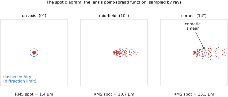
fig-spot-diagram · spot diagram = the lens's PSF sampled by rays: 3 field positions (on-axis tight → corner comatic smear), RMS spot µm under each, dashed Airy (diffraction) circle (Lens optimization) ✅fig-spot-diagram · spot diagram = the lens's PSF sampled by rays: 3 field positions (on-axis tight → corner comatic smear), RMS spot µm under each, dashed Airy (diffraction) circle (Lens optimization) ✅fig-wb-before-after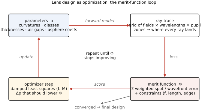
fig-merit-function-loop · lens design as optimization, a closed loop: parameters → ray-trace (fields × wavelengths × pupil zones) → merit function Φ (weighted spot/wavefront + constraints) → damped-least-squares step → repeat; the book's forward-model+loss+optimizer pattern (Lens optimization) ✅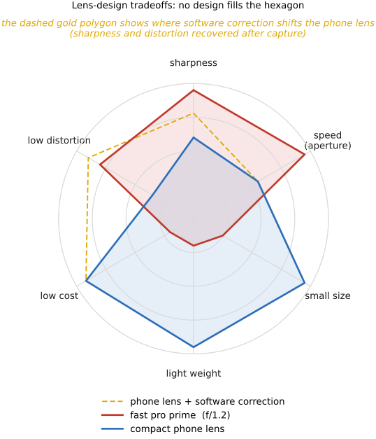
fig-lens-design-tradeoff · lens-design Pareto cartoon as a 6-axis radar (sharpness, speed, size, weight, cost, distortion): fast pro prime vs compact phone lens overlaid, plus a dashed polygon showing where software correction shifts the phone lens (Lens optimization) ✅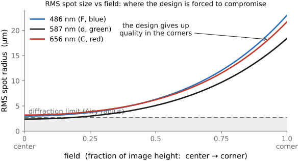
fig-rms-spot-vs-field · RMS spot radius (µm) vs field (center→corner) for 3 wavelengths, rising toward the edge, with the Airy diffraction limit as a shaded dashed floor (Lens optimization) ✅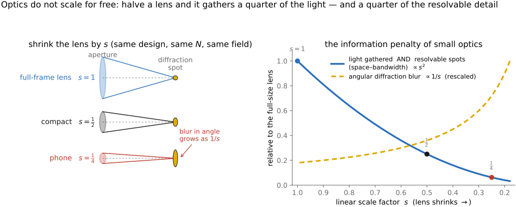
fig-optics-scaling-law · 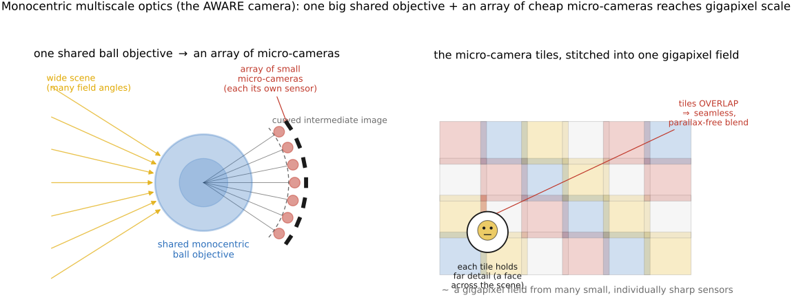
fig-monocentric-multiscale · 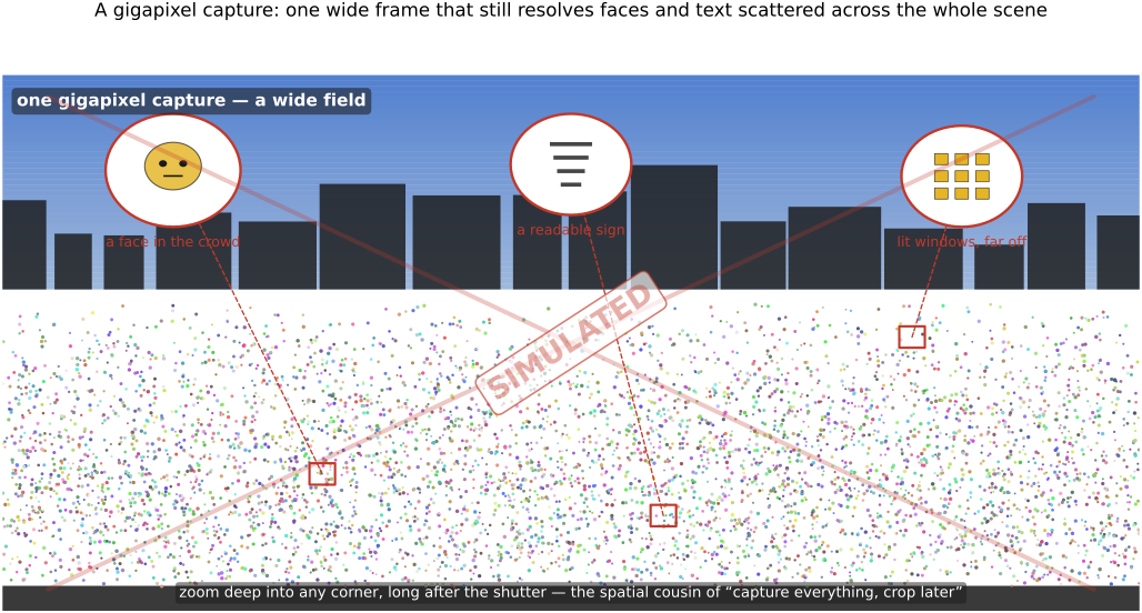
fig-gigapixel-mosaic · 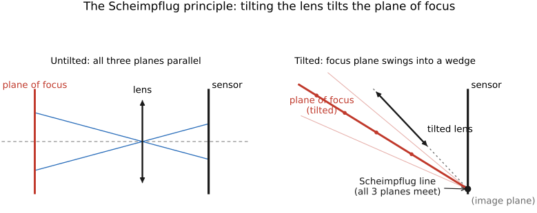
fig-scheimpflug-tilt · the Scheimpflug principle: tilting the lens makes the lens plane, image plane & plane of focus meet in a common line → the focus plane tilts into a wedge of sharpness; contrasted with the parallel (untilted) case ✅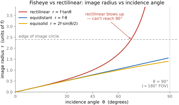
fig-fisheye-projection · projection mappings — image radius r vs incidence angle θ for rectilinear (r=f·tanθ, blows up near 90°), equidistant (r=f·θ) and equisolid (r=2f·sin(θ/2)); why fisheye reaches ~180° where rectilinear can't ✅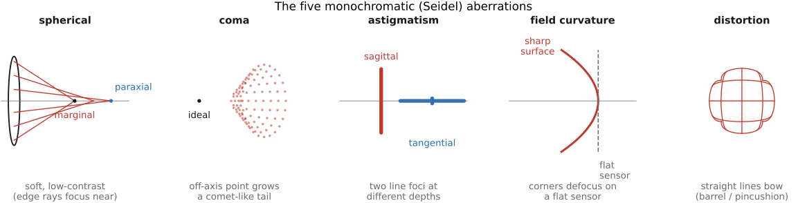
fig-seidel-aberrations · the five monochromatic (Seidel) aberrations at a glance — spherical, coma, astigmatism, field curvature, distortion — each a tiny ray/spot icon + a one-line "what it looks like" note ✅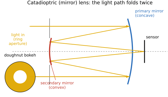
fig-catadioptric-mirror-lens · a mirror (catadioptric) lens: light folds via primary + secondary mirror (Cassegrain); central obstruction → ring-shaped (doughnut) bokeh — folded path + doughnut-highlight inset ✅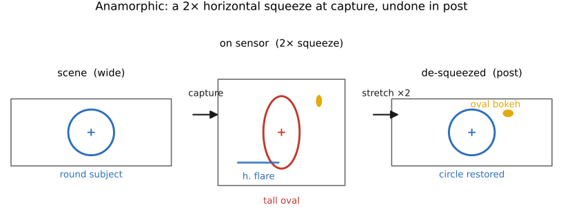
fig-anamorphic-squeeze · anamorphic optics: 2× horizontal squeeze at capture → de-squeeze in post; a circle → vertical oval on sensor → restored; oval bokeh + horizontal flares noted ✅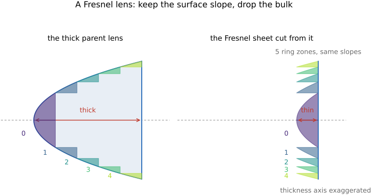
fig-fresnel-zones · a Fresnel lens: collapse a thick convex lens into concentric ring "zones" that keep the local surface slope but drop the bulk; cross-section of a normal lens vs its Fresnel equivalent ✅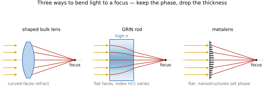
fig-grin-vs-metalens · three ways to bend light: shaped bulk lens (refraction), a GRIN rod (curved ray through a varying-index medium, flat faces), and a metalens (flat surface, sub-wavelength nanostructures setting a phase profile); "keep the phase, drop the thickness" ✅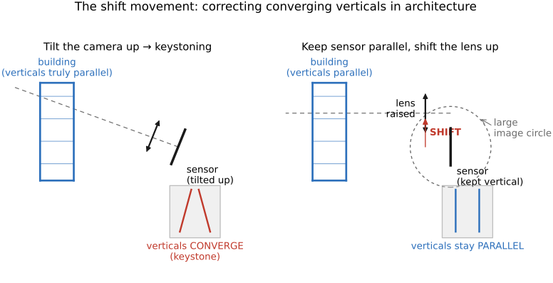
fig-tilt-shift-perspective · the *shift* movement (not tilt): tilting the camera up keystones a building (converging verticals) vs. keeping the sensor vertical/parallel and raising the lens within a large image circle, so verticals stay parallel — architectural perspective control ✅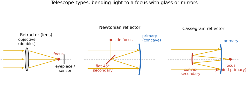
fig-telescope-types · refractor (doublet objective → focus) vs. reflectors — Newtonian (concave primary + flat 45° secondary → side focus) and Cassegrain (primary + convex secondary → focus through a hole behind the primary); glass vs. mirrors to a focus ✅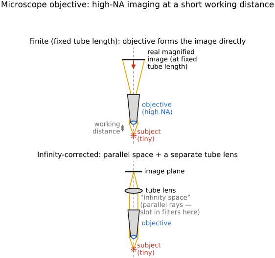
fig-microscope-objective · high-NA objective at a short working distance: finite (fixed tube length, objective forms the image directly) vs. infinity-corrected (subject at front focus → parallel "infinity space" → separate tube lens forms the image) ✅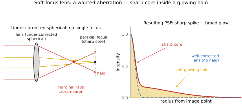
fig-soft-focus · a soft-focus portrait lens: under-corrected spherical aberration (marginal rays cross nearer than paraxial → halo at the paraxial plane) and the resulting PSF — a sharp core inside a broad glow vs. a well-corrected lens; a *wanted* aberration ✅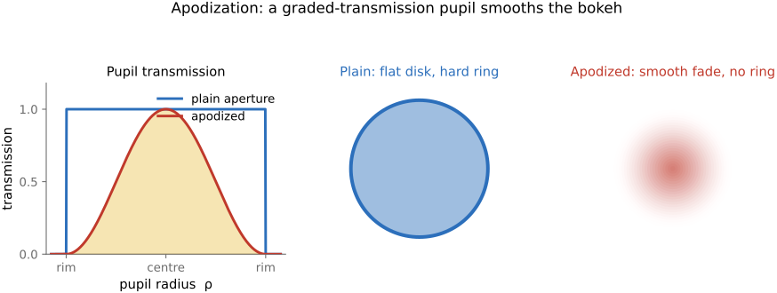
fig-apodization-pupil · an apodizing filter: pupil transmission profile (hard-edged plain aperture vs. radially graded) → the defocus disk each makes (flat disk with a hard ring vs. a smoothly fading disk, no ring) — shaping the bokeh PSF in hardware ✅fig-fresnel-zones · a Fresnel lens: collapse a thick convex lens into concentric ring "zones" that keep the local surface slope but drop the bulk; cross-section of a normal lens vs its Fresnel equivalent ✅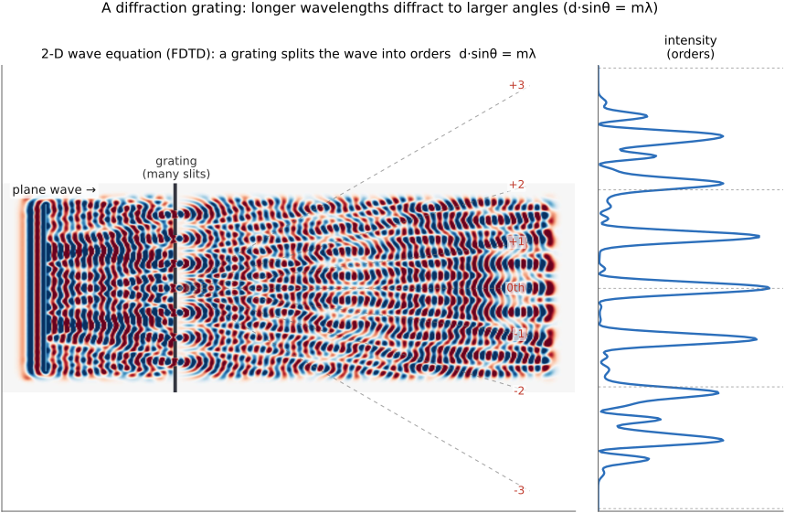
fig-diffraction-grating-sim · live 2-D FDTD wave sim of a **diffraction grating** (many slits): plane wave splits into orders along d·sinθ=mλ, orders sweep with wavelength (longer λ → larger deviation); intensity comb peaks at the orders (OPTICS → Diffractive elements) ✅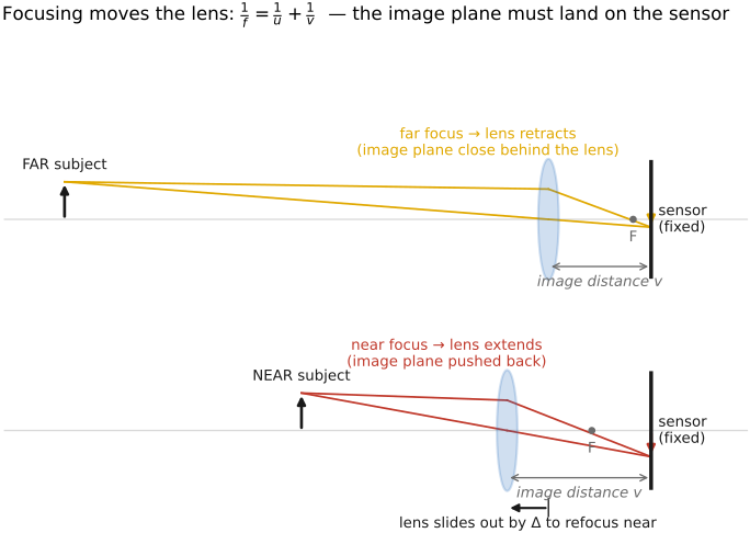
fig-focus-conjugate-move · focusing geometry: as subject distance u changes the image distance v must change (1/f=1/u+1/v); the lens slides to keep the image plane on the fixed sensor — near vs far focus (lens extends vs retracts) ✅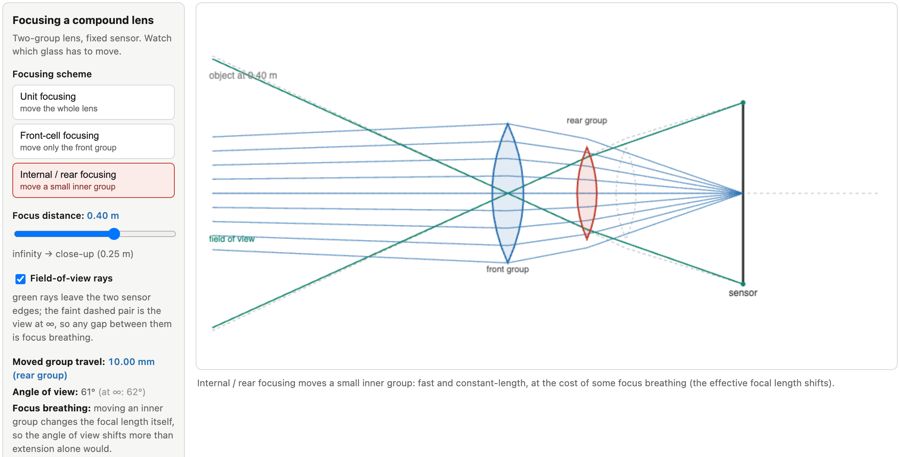
fig-compound-focusing · **interactive** (10.8 Focus): 2-D ray trace of a two-group lens on a fixed sensor; mode selector unit / front-cell / internal focusing + a focus-distance slider (∞→0.25 m); highlights which group moves, its travel, and the focus-breathing tradeoff ✅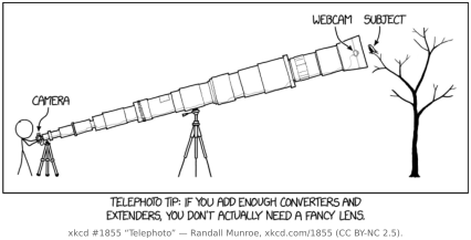
fig-xkcd-1855 · 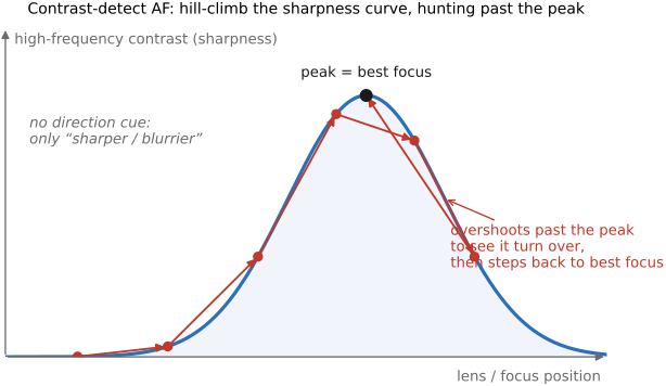
fig-contrast-af-curve · contrast-detect AF: high-frequency contrast (sharpness) vs focus position, peaked at best focus; hill-climb arrows that must overshoot past the peak then step back (no direction cue) ✅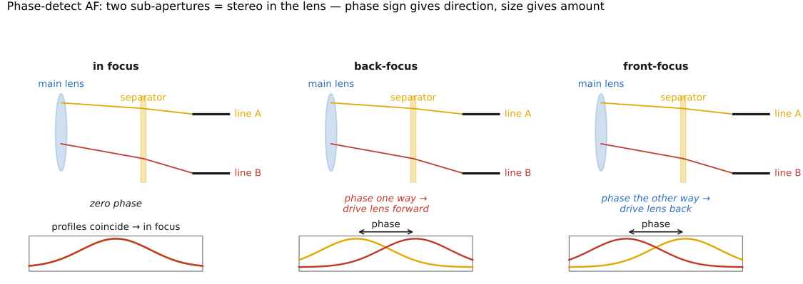
fig-pdaf-principle · phase-detect AF: a separator splits the beam to two line sensors; the signed phase (separation) of the two profiles gives direction + amount of defocus ("stereo in the lens"); in-focus vs front/back-focus ✅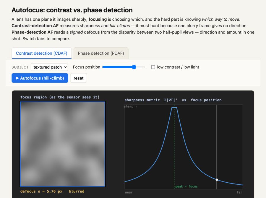
fig-autofocus-demo · **interactive** autofocus (9.6 Focus, autofocus): CDAF tab — sharpness ∑‖∇I‖² vs focus, hill-climb with hunting + low-light failure; PDAF tab — two half-pupil line signals, signed disparity → one-shot focus ✅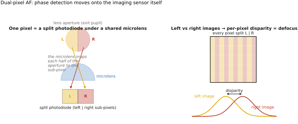
fig-dual-pixel-af · on-sensor / dual-pixel AF: a photodiode split into L/R halves under one microlens; the L vs R images give per-pixel disparity → defocus; split-pixel cross-section + the two readout images ✅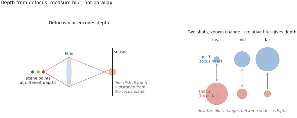
fig-depth-from-defocus · depth from defocus: the blur-disk diameter grows with distance from the focus plane; two shots at different focus/aperture → estimate depth from the relative blur ✅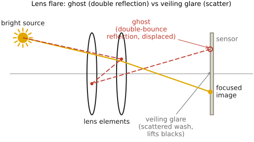
fig-lens-flare-ghosting · stray light: a bright source, a ray reflecting off two internal lens surfaces → a "ghost" landing displaced on the sensor, plus a veiling-glare wash; ghost vs flare labeled ✅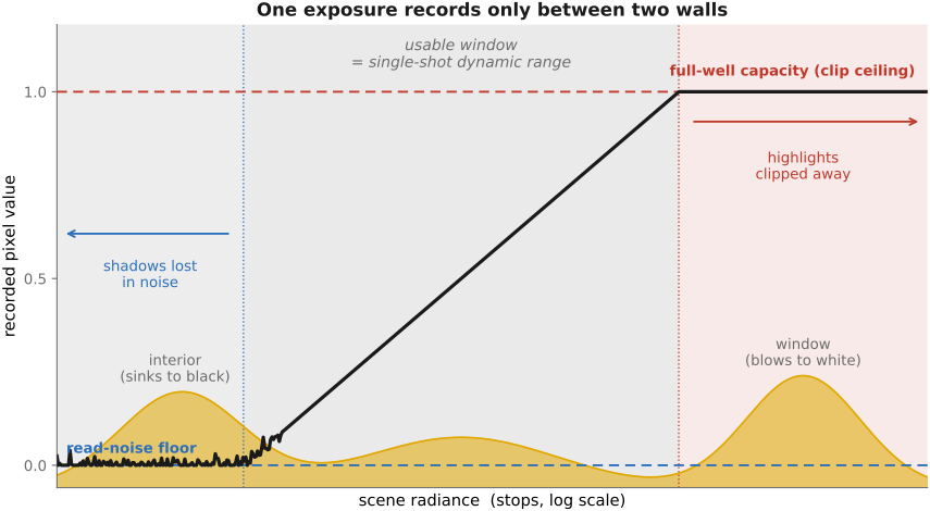
fig-dr-clip-vs-noise · one exposure's two walls — clipping at full-well above, the noise floor below — shading the narrow band of scene contrast that fits between them 🟨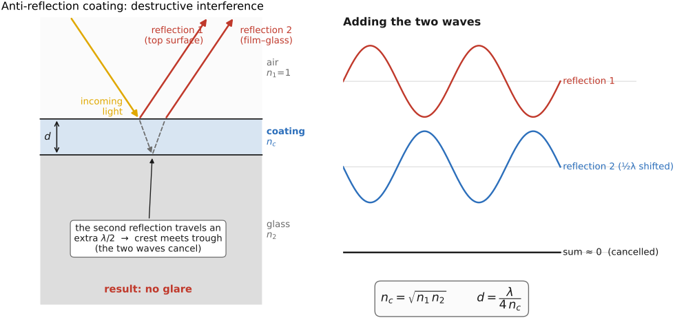
fig-ar-coating-interference · anti-reflection coating: a quarter-wave film cancels the front-surface reflection by destructive interference (top-surface reflection vs film–glass reflection, extra path λ/2 → out of phase); two emergent wavelets summing to ~0 + design rules $n_c=\sqrt{n_1 n_2}$, $d=\lambda/4n_c$ ✅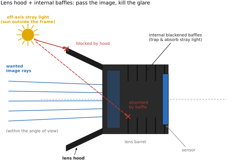
fig-lens-hood-baffles · lens hood + internal blackened baffles: an off-axis source (sun outside the frame) is blocked by the hood; stray light that sneaks in is trapped/absorbed by baffles; wanted image-forming rays (within the angle of view) pass through to the sensor ✅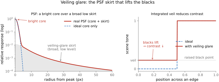
fig-veiling-glare-psf · a PSF with a bright core + a broad low-level skirt (veiling glare) on a log-radial profile; second panel shows the integrated veil lifting blacks / reducing contrast ✅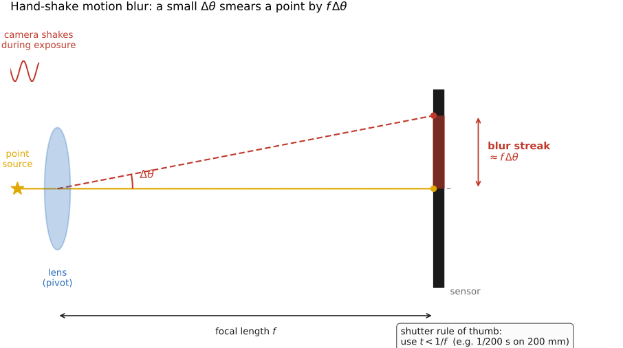
fig-handshake-motion-blur · hand-shake motion blur: a small angular shake $\Delta\theta$ over the exposure smears a point into a streak of length $\approx f\,\Delta\theta$ on the sensor (lens as pivot, focal length $f$); the $t<1/f$ shutter rule of thumb ✅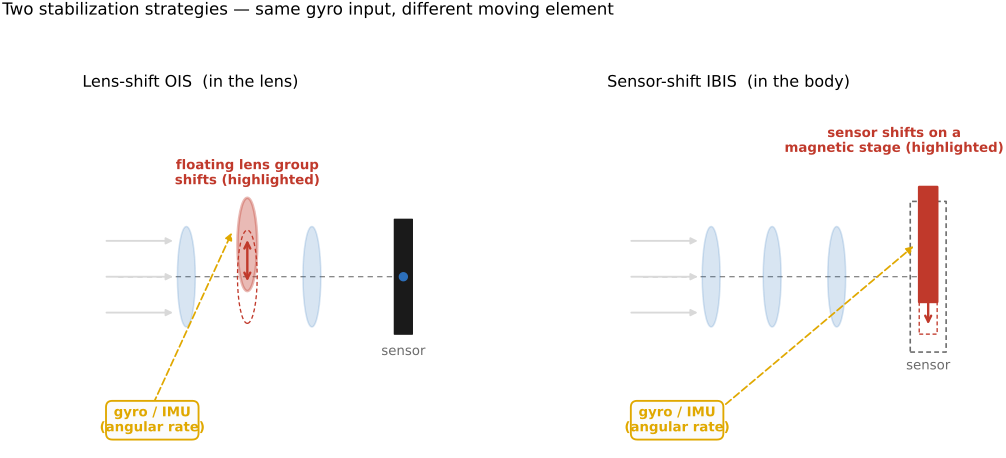
fig-ois-vs-ibis · two stabilization strategies side-by-side: lens-shift OIS (floating lens group moves) vs sensor-shift IBIS (sensor moves on a magnetic stage), moving element highlighted, same gyro/IMU input ✅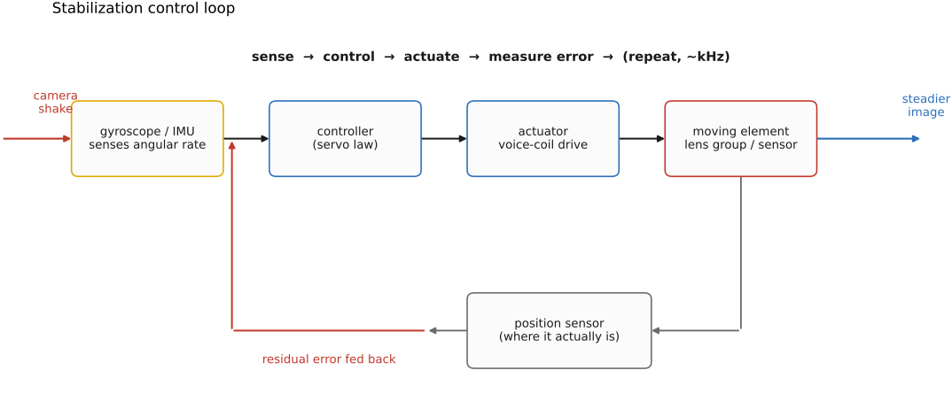
fig-gyro-feedback-loop · the stabilization control loop as a block diagram: gyro/IMU senses angular rate → controller → actuator moves the lens group/sensor → position sensor feeds residual error back (sense→control→actuate→measure, ~kHz) ✅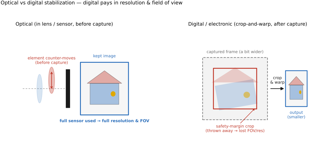
fig-digital-vs-optical-stab · optical (in lens/sensor, before capture, full resolution & FOV) vs digital/electronic IS (crop-and-warp in software after capture): the EIS safety-margin crop + warp costing resolution/field of view vs the optical in-lens/sensor correction ✅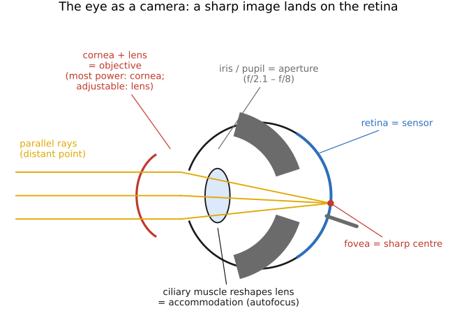
fig-eye-as-camera · the eye as a camera: cornea + crystalline lens = objective, iris/pupil = aperture, retina = sensor (fovea), accommodation = autofocus — labeled cross-section ✅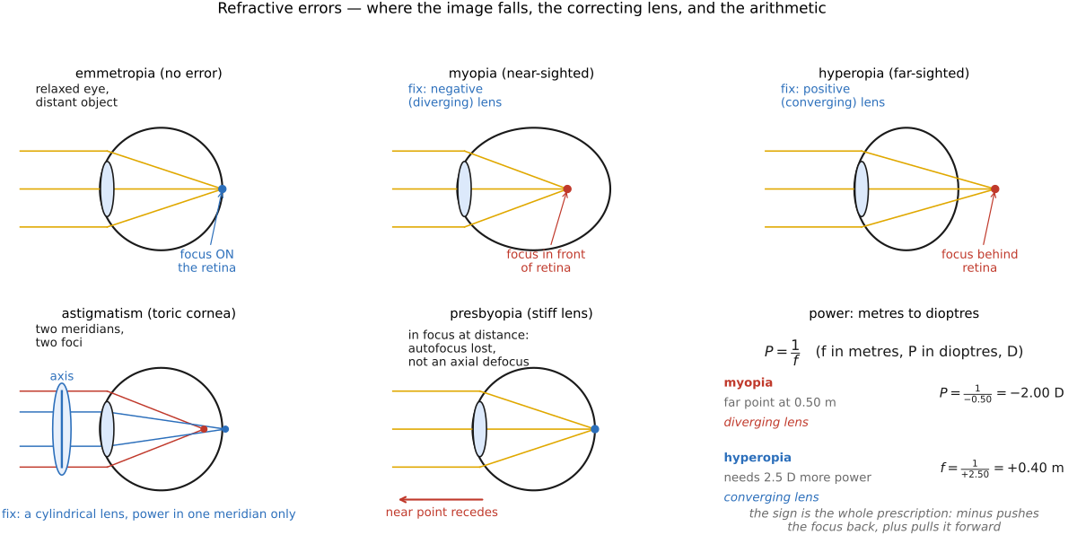
fig-refractive-errors · the four refractive errors — myopia / hyperopia / astigmatism / presbyopia — where the image focuses vs the retina and the correcting (negative / positive / cylindrical / add) lens ✅fig-bifocal-progressive-af