Computational Photography, an AI-powered Slopendium — 15 Demosaicking and joint methods

▸15.1 Basic traditional demosaicking⧉

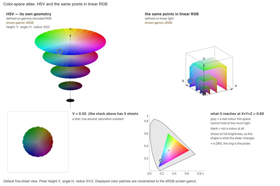
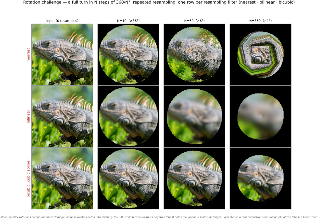
`fig-color-space-atlas` · **interactive** color-space atlas: one space drawn twice, in its own geometry (cube / cone / bi-cone / warped cube) and in a chosen ambient frame (XYZ, LMS, linear RGB, sRGB, Chong, Oklab), from the same lattice, as edges / voxels / one slice; MacAdam ellipses optional; click to read coordinates in both; stripes for colors outside sRGB. Placed at the end of the perceptually-uniform section of **4.6 Advanced color**, where it works as the chapter's capstone: by then HSV/HSL, CIELAB, Oklab and Chong have each been shown alone, and the atlas is about the map between them. URL carries the state (`?space=&ambient=&mode=&axis=&at=&grid=&macadam=&zebra=`). 🟨

`fig-rotation-challenge` · Andrew Adams' rotation challenge: rotate a full turn in N steps of 360/N° (each step bilinear-resamples the PREVIOUS result), for N∈{10,60,360}; track a validity mask through identical rotations so corners that ever leave the frame go black. Result returns to 0° but is resampled N times → accumulated blur/mush + shrinking valid region toward the inscribed disc. More, smaller rotations compound MORE damage (rotate k× by 360/N, not once by k·360/N) ✅

equations

the bilinear estimate

the constant-difference assumption $R - G$ locally smooth

the Hamilton-Adams gradient test.

15.1.1 Downsampling and bilinear interpolation, and how they fail⧉

15.1.2 Interpolate along the edge, not across it⧉

15.1.3 Interpolate differences, not channels⧉

15.1.4 Demosaicking and other aspects of imaging⧉

▸15.2 Advanced traditional demosaicking⧉

15.2.1 Adaptive homogeneity-directed demosaicking (AHD)⧉

15.2.2 Residual interpolation and ARI⧉

15.2.3 Demosaicking as demultiplexing: frequency-domain methods⧉

15.2.4 Where the classical methods stop⧉

▸15.3 Mosaics and aliasing⧉

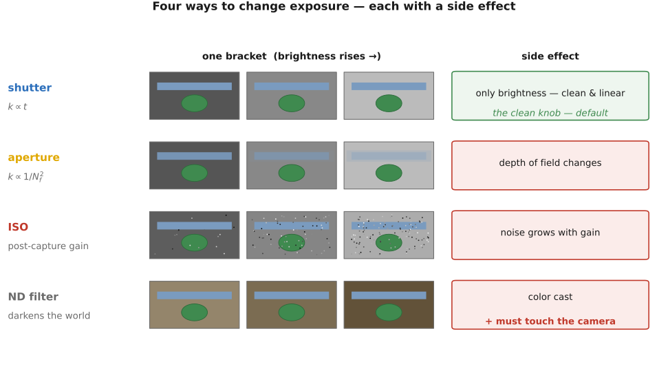
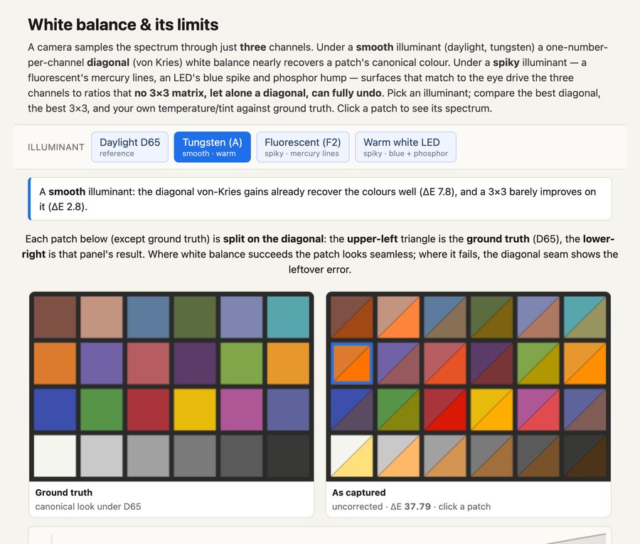
`fig-vary-exposure-knobs` · the four exposure knobs and their side effects — none for shutter, depth-of-field for aperture, noise for ISO, color cast plus camera contact for ND 🟨

`fig-white-balance` · **interactive** white-balance / metamerism playground (BASIC → the limits of white balance): a Macbeth ColorChecker rendered from spectral reflectances under a chosen illuminant (D65 / tungsten A / spiky fluorescent / warm LED); shows captured vs D65 ground truth, each patch's resulting spectrum, the best **diagonal** (von Kries) vs full **3×3** correction (least-squares, mean ΔE printed), and manual temperature/tint sliders — spiky illuminants leave an irreducible residual no 3×3 can remove ✅

⬜ figure not yet created

the prefilter mismatch on Bayer

⬜ figure not yet created

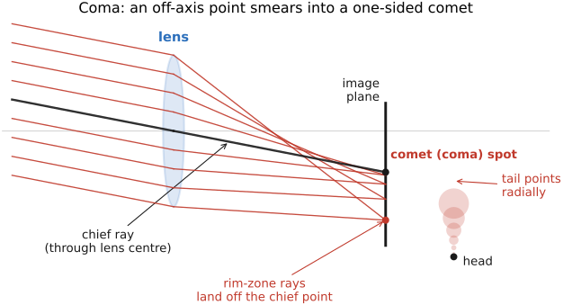
router footprints as prefilters

`fig-coma` · coma: an off-axis parallel bundle where each annular aperture zone images to a different height; chief ray through the lens center + zonal rays missing a common focus → the one-sided comet ("coma") spot with a head and a radial tail ✅

15.3.1 Each channel lives on a sparser lattice⧉

15.3.2 All channels at once: luma and chroma⧉

15.3.3 False color and moiré as spectral overlap⧉

15.3.4 X-Trans, Quad-Bayer and Nona-Bayer in the Fourier domain⧉

15.3.5 Prefiltering a mosaic: one blur for three lattices⧉

15.3.6 Anti-aliasing filters are disappearing⧉

15.3.7 Nano-prisms as anti-aliasing filters⧉

▸15.4 Optimizing and searching classical demosaickers⧉

15.4.1 Fitting a classical demosaicker by gradient descent⧉

15.4.2 Searching for the program itself⧉

▸15.5 Alternative color filter arrays⧉

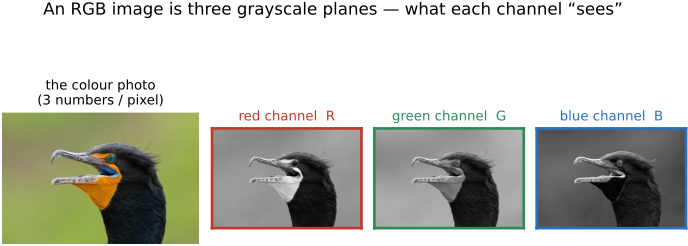
`fig-rgb-channels` · a real photo split into its R / G / B grayscale planes — what each channel "sees" (Image representation → An image is an array, BASIC) ✅

15.5.1 Fuji's X-Trans⧉

15.5.2 Quad-Bayer and its modes⧉

15.5.3 RGBW and sparse color⧉

15.5.4 Designing the array and the algorithm together⧉

▸15.6 Learned demosaicking⧉

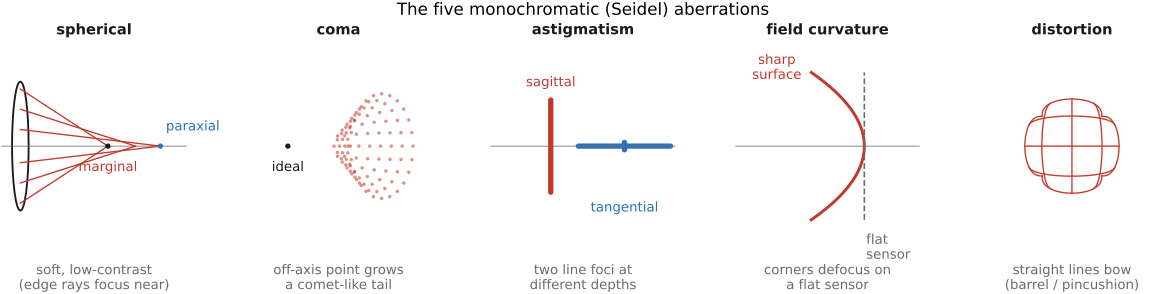
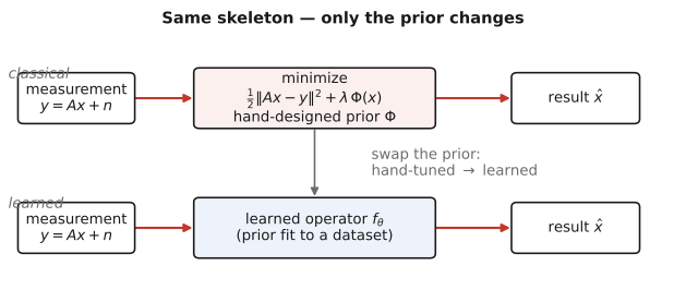
`fig-seidel-aberrations` · the five monochromatic (Seidel) aberrations at a glance — spherical, coma, astigmatism, field curvature, distortion — each a tiny ray/spot icon + a one-line "what it looks like" note ✅

`fig-learned-vs-handdesigned` · same inverse-problem skeleton, prior swapped: classical (data-fit + hand prior $\Phi$) vs learned ($f_\theta$ fit to data) (ML) ✅

15.6.1 The data problem hiding inside a free training set⧉

15.6.2 Architectures, briefly⧉

15.6.3 Unrolling, and the bridge from the classical formulation⧉

15.6.4 What the networks learned⧉

15.6.5 Benchmarks and their age⧉

▸15.7 Neighboring problems in the raw stage⧉

15.7.1 Defective pixels⧉

15.7.2 Phase-detect autofocus pixels⧉

15.7.3 Black level, clipping, and where pink highlights come from⧉

15.7.4 Lens shading and crosstalk⧉

15.7.5 The ordering claim, once more⧉

▸15.8 Joint demosaicking and denoising⧉

equations

the joint forward model $y = M(x) + n$ with $M$ the mosaic operator and $n$ signal-dependent

the sequential pipelines written out for comparison.

15.8.1 The two orderings, made visible⧉

15.8.2 The joint formulation⧉

15.8.3 FlexISP: one energy, one prior⧉

15.8.4 What it buys, and where it is deployed⧉

15.8.5 Correcting chromatic aberration jointly⧉

15.8.6 The argument generalizes⧉

▸15.9 Joint methods and the end-to-end pipeline⧉

⬜ figure not yet created

the two pipelines drawn side by side with the adjustable parameters marked, which is the whole argument in one picture. fig-tonemap-study-disagreement

15.9.1 What end-to-end learning gains⧉

15.9.2 What it costs⧉

15.9.3 Keeping a useful intermediate representation⧉

15.9.4 Where the field actually is⧉

15.9.5 Where demosaicking sits in the pipeline⧉

▸15.10 Quad-Bayer and Nona-Bayer processing⧉

15.10.1 Why the classical methods do not transfer⧉

15.10.2 Remosaicking: making the sensor look like Bayer⧉

15.10.3 Demosaicking the grouped layout directly⧉

15.10.4 Remosaic or demosaic directly?⧉

15.10.5 Split exposures within a block⧉

▸15.11 Synthetic data, unprocessing, and raw reconstruction⧉

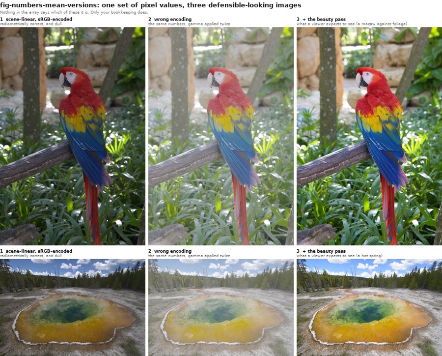
`fig-numbers-mean-versions` · one set of raw-DNG pixel values rendered three plausible ways — scene-linear→sRGB (dull but correct) · the same numbers mis-encoded (double gamma) · + beauty pass (what a viewer expects); makes "numbers are meaningless without their encoding" concrete (Image representation → what the numbers mean, BASIC) ✅

equations

the forward pipeline as a composition and its inverse, with the non-invertible steps named.

15.11.1 The inversion, step by step⧉

15.11.2 Why an approximate inverse is good enough⧉

15.11.3 Raw reconstruction as a goal of its own⧉

15.11.4 The pipeline diagram, walked backwards⧉

▸15.12 Hardware alternatives to the mosaic⧉

fig-pixel-shift · Bayer + sensor pixel-shift hybrid: four one-photosite-shifted Bayer frames → merged full RGB per pixel, no demosaicking (half-pixel shift → super-resolution) ✅

15.12.1 Pixel shift: spending time, precisely⧉

15.12.2 Foveon and stacked photodiodes: spending silicon depth⧉

15.12.3 Assorted pixels: spending spatial resolution on another axis⧉

15.12.4 RGB-NIR: adding a band the eye does not have⧉

15.12.5 Color wheels: spending time, sequentially, for many bands⧉

15.12.6 Four ways to multiplex color⧉

15.12.7 Routing color instead of filtering it⧉

15.12.8 One table, one question⧉

15.13 Demosaicking TLDR⧉