BookNotesSlidesP-sets Syllabusdraft · v0.2.49.1
💬Comments welcome. To leave a note, select any text and click the note / highlight button that pops up — or open the panel with the tab at the top-right (‹). Notes are visible only inside our private review group.
Computational Photography, an AI-powered Slopendium — 34 Computational sensors
expand to📖 Full book outline1 parts · 12 chapters · 66 sections · 21 figures embedded · 3 placeholders · double-click a figure to enlarge
▸Part 34 COMPUTATIONAL SENSORS⧉
<!--uid: computational-sensors-->
The sensor is the other place to be clever: instead of (or as well as) coding the optics, build pixels that measure something an ordinary Bayer sensor throws away — range, photon arrival time, velocity, change events — or fuse in data from sensors that are not cameras at all. This part collects the **computational sensor** ideas, the **extra (non-visual) sensors** that ride along in a modern device, and the **high-/ultra-high-speed temporal** capture that lives most naturally with them.
▸34.1 Assorted pixels⧉
34.1.1 Dual-pixel and phase-detect pixels: buying depth and focus⧉
34.1.2 Clear, white, and other color-filter variants⧉
34.1.3 Polarization pixels⧉
34.1.4 Spatially varying exposure: assorting for dynamic range⧉
34.1.5 The common thread⧉
▸34.2 Modern sensors (quad Bayer, in-sensor HDR, and beyond)⧉
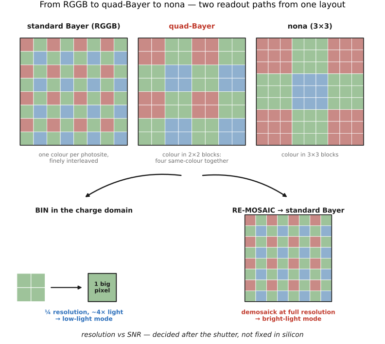
fig-quad-bayer-layout
fig-quad-bayer-layout ·
⬜ figure not yet created
binning vs remosaic paths)
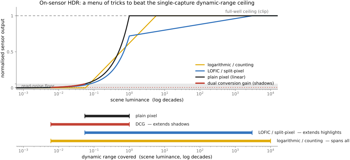
fig-insensor-hdr-methods
fig-insensor-hdr-methods ·
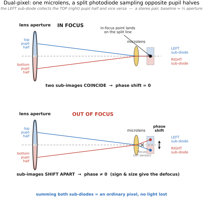
fig-dual-pixel-split
fig-dual-pixel-split ·
34.2.1 Quad Bayer, Tetracell, and nona-binning⧉
34.2.2 In-sensor HDR: capturing range before the merge⧉
34.2.3 Dual-pixel autofocus, on the same sensor⧉
34.2.4 BSI and stacked sensors: compute under the pixels⧉
34.2.5 The global-versus-rolling shutter trade⧉
34.2.6 Beyond: nano-prism, organic, and event pixels⧉
▸34.3 On-sensor HDR⧉
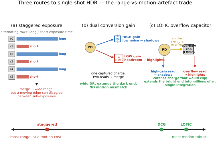
fig-onsensor-hdr-strategies
fig-onsensor-hdr-strategies ·
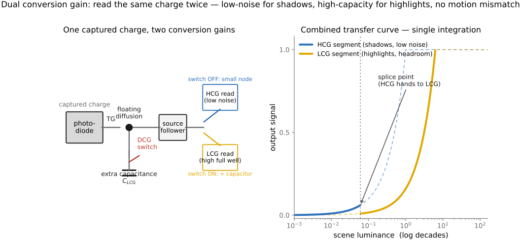
fig-dual-conversion-gain
fig-dual-conversion-gain ·
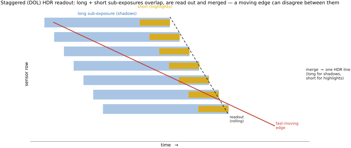
fig-staggered-exposure-readout
fig-staggered-exposure-readout ·
34.3.1 Staggered / multiple-exposure readout (DOL-HDR)⧉
34.3.2 Dual (and triple) conversion gain (DCG)⧉
34.3.3 Split-pixel: a large and a small photodiode⧉
34.3.4 Spatially-varying exposure (SVE) / assorted exposures⧉
34.3.5 Lateral overflow integration capacitor (LOFIC)⧉
34.3.6 Logarithmic, self-resetting, and counting pixels⧉
34.3.7 On-sensor HDR versus multi-frame HDR⧉
▸34.4 Depth sensors⧉
• a taxonomy of ways to recover per-pixel **range $Z$** — the dimension a single camera throws away in the divide-by-$Z$ projection (FUNDAMENTALS):
• **stereo** (passive): two cameras a baseline $B$ apart; triangulate depth from **disparity**, $Z = fB/d$ (cross-ref *Multiple view geometry*). Cheap and passive, but fails on **textureless / repetitive** surfaces — the correspondence problem.
• **stereo with structured light** (active): *project* a known pattern — stripes, a pseudo-random **speckle / dot** pattern, or phase-shifted sinusoids — so correspondence is solved even on a blank wall; one camera + one projector triangulate. The original **Kinect v1** (PrimeSense speckle); industrial **phase-shift profilometry** for 3-D scanning. Robust indoors; struggles in bright sun and on specular / very dark surfaces.
• **LiDAR** (light detection and ranging): emit a laser pulse and time its return (**direct time-of-flight**) for each scanned or flashed direction → a depth **point cloud**. Scanning (spinning or MEMS-mirror) vs **flash** LiDAR (a SPAD array — cross-ref single-photon sensors below); long range, works in the dark — the basis of self-driving range sensing and recent phone/tablet LiDAR.
• **time-of-flight** (the other active route): continuous-wave (**phase**) ToF — e.g. **Kinect v2** — vs direct/pulsed ToF (LiDAR); see the Time-of-flight subsection below.
• others, in passing: depth from **focus / defocus** and **dual-pixel** (Optics — Focus/AF), **monocular learned depth** (COMPUTATIONAL TOOLS — Deep learning), and shape-from-X.
34.4.1 Stereo: passive triangulation⧉
34.4.2 Structured light: projecting the texture⧉
34.4.3 LiDAR and direct time-of-flight⧉
34.4.5 Passive depth from one camera, in passing⧉
34.4.6 The menu, in one view⧉
▸34.5 Single-photon sensors (SPAD, avalanche, photon counting)⧉
34.5.1 From avalanche gain to a single-photon click⧉
34.5.2 Photon-counting arrays: zero read noise, shot-noise-limited⧉
34.5.3 The Quanta Image Sensor: a different road to one photon⧉
34.5.4 What it costs: dark counts, dead time, fill factor, data rate⧉
▸34.6 Doppler / velocity imaging⧉
• per-pixel **velocity** from a frequency / phase shift — optical Doppler, Doppler **lidar / radar**, laser **vibrometry**; the imaging cousin of medical **Doppler ultrasound** and Doppler weather radar
• measures motion **directly** (radial velocity) rather than inferring it from frame-to-frame optical flow → fast, robust in low light; pairs with ToF (range + range-rate)
34.6.1 The Doppler shift, as a velocity sensor⧉
34.6.2 The instruments: vibrometry, Doppler LiDAR, radar⧉
34.6.3 Where it fits⧉
▸34.7 Event sensors⧉
34.7.1 How it works: per-pixel change detection⧉
34.7.2 The upside: microseconds, dynamic range, no blur, little data⧉
34.7.3 The downside: no picture, and a new kind of data⧉
34.7.4 Uses, lineage, and the contrast with single-photon⧉
▸34.8 Specialized and research sensors⧉
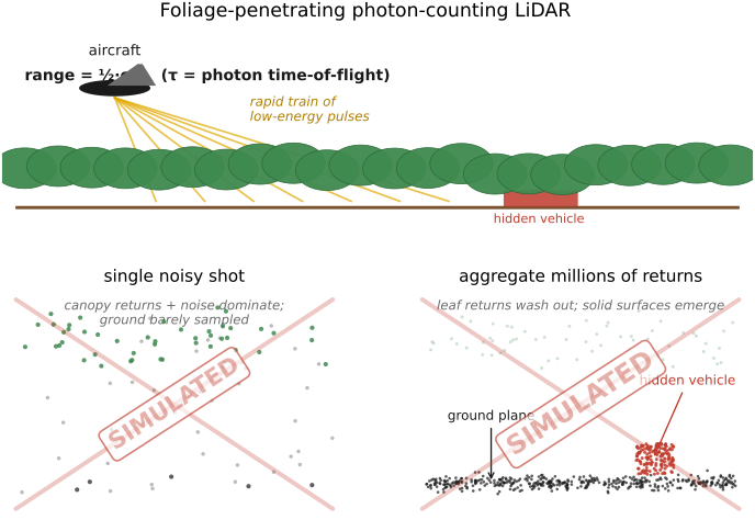
fig-geiger-apd-lidar
fig-geiger-apd-lidar ·
34.8.1 Geiger-mode avalanche-photodiode arrays: photon-counting laser radar⧉
34.8.2 Digital-pixel focal-plane arrays⧉
34.8.3 Scientific imagers: cryogenic CCDs, sCMOS, and gigapixel mosaics⧉
34.8.4 Stacked and processing-in-pixel sensors⧉
34.8.5 Curved focal planes⧉
34.8.6 Beyond the visible, and filter-array sensors⧉
34.8.7 Radiation-hardened and defense focal planes⧉
34.8.8 The chapter's point⧉
▸34.9 Extra sensors and non-visual data⧉
34.9.1 Accelerometer and gyroscope: the inertial measurement unit⧉
34.9.2 Sound: microphones, audio-visual sync, and the visual microphone⧉
34.9.3 GPS: geotagging and place⧉
34.9.4 Compass and magnetometer: heading and orientation⧉
34.9.5 Near-infrared: the cut filter, dark flash, and NIR-assisted denoise⧉
34.9.6 Temperature: dark-current compensation⧉
34.9.7 Accelerometer, gyro⧉
34.9.8 Sound⧉
34.9.9 GPS⧉
34.9.10 Compass⧉
34.9.11 Near IR⧉
34.9.12 Temperature⧉
▸34.10 Ultra high-speed imaging⧉
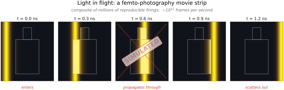
fig-light-in-flight
fig-light-in-flight ·
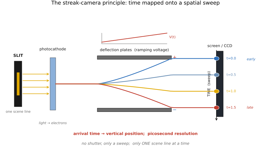
fig-streak-camera
fig-streak-camera ·
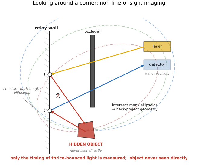
fig-ultrafast-nlos
fig-ultrafast-nlos ·
34.10.1 Streak cameras: sweeping time onto a spatial axis⧉
34.10.2 Femto-photography: a movie of light in flight⧉
34.10.3 Compressive ultrafast photography: a single-shot coded streak⧉
34.10.4 Transient imaging and looking around corners⧉
34.10.5 The bridge to direct time-of-flight and LiDAR⧉
▸34.11 Hyperspectral imaging, color wheels⧉
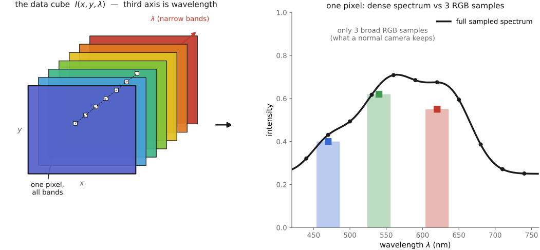
fig-hyperspectral-cube
fig-hyperspectral-cube · the cube as an image stack indexed by wavelength, contrasting a pixel's full spectrum against the three numbers RGB retains 🟨
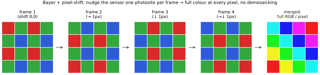
fig-pixel-shift
fig-pixel-shift · Bayer + sensor pixel-shift hybrid: four one-photosite-shifted Bayer frames → merged full RGB per pixel, no demosaicking (half-pixel shift → super-resolution) ✅
fig-hyperspectral-rgb-vs-spectrum
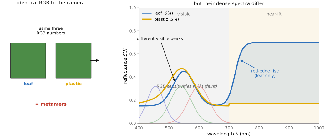
fig-hyperspectral-rgb-vs-spectrum · two materials identical in RGB but clearly distinct in their measured reflectance spectra (with the three RGB sensitivities overlaid) — the metamer case for many bands 🟨
fig-hyperspectral-capture
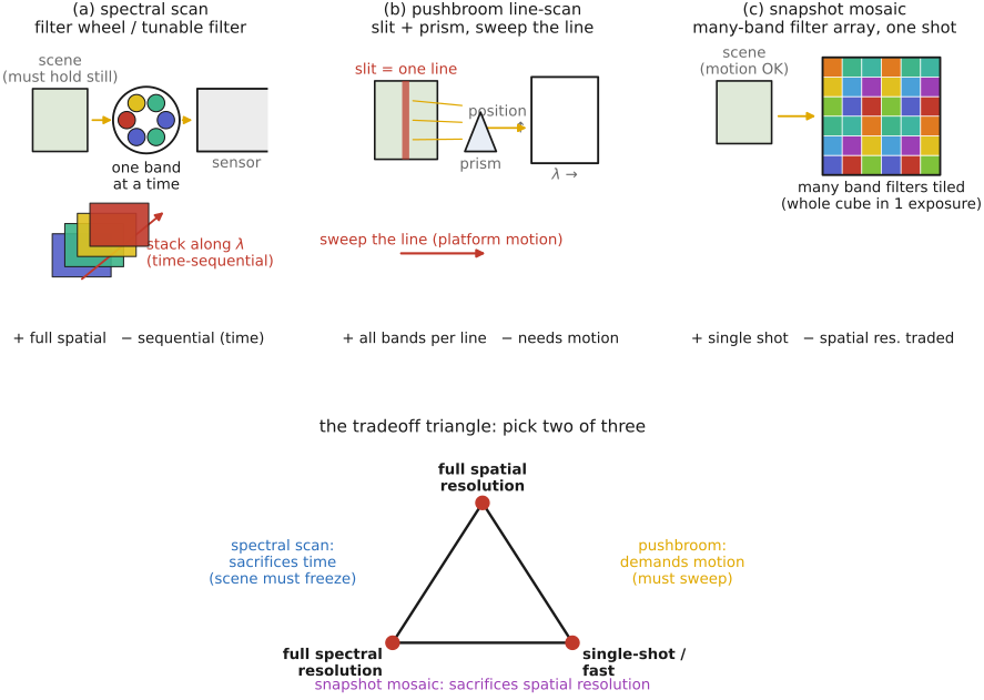
fig-hyperspectral-capture · the three capture architectures (spectral scan, pushbroom line-scan, snapshot mosaic) and the spatial-vs-spectral-vs-time tradeoff triangle 🟨
⬜ figure not yet created
pushbroom slit+prism scanning lines in space
fig-demosaick-snapshot
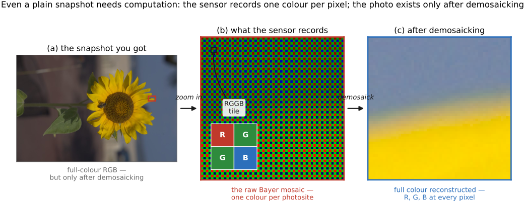
fig-demosaick-snapshot · even a plain snapshot needs computation: one color per pixel (Bayer mosaic) → demosaicked RGB ✅
⬜ figure not yet created
`fig-hyperspectral-uses` (material map / NDVI vegetation map / art-conservation pigment or underdrawing reveal). fig-hyperspectral-uses
💡 **Big lesson (L11.2 · Capture the full set, decide later — wavelength axis):** RGB throws away the spectrum at the instant of capture (three broad bands, irreversibly mixed). Hyperspectral imaging **records the whole spectrum per pixel and decides spectral questions afterward** — the same defer-the-decision move as HDR (exposure axis), focal stacks (focus axis) and light fields (aperture axis), now on the **wavelength axis**. Cost: data, light, capture time. Payoff: you can ask *what is this made of* long after the shutter. (→ see Big lesson **L11.2**, [[Big Lessons]]; first-appearance box at the light-field introduction.)
equations
**measurement as projection** — a camera channel $c$ records $I_c(x,y)=\int S(x,y,\lambda)\,R_c(\lambda)\,d\lambda$
RGB is this with **3** broad $R_c$
hyperspectral is the same with **many narrow** band responses $R_b(\lambda)$ (near-delta), recovering the spectrum $S(x,y,\lambda)$ sampled at the bands — i.e. the cube $I(x,y,\lambda_b)$
**NDVI** $=\dfrac{I_{\mathrm{NIR}}-I_{\mathrm{red}}}{I_{\mathrm{NIR}}+I_{\mathrm{red}}}$ (a band ratio — a per-pixel multiplicative/normalized index, L2.6).
▸34.12 Polarization imaging⧉
fig-polarization-axis
fig-polarization-axis ·
fig-seasons
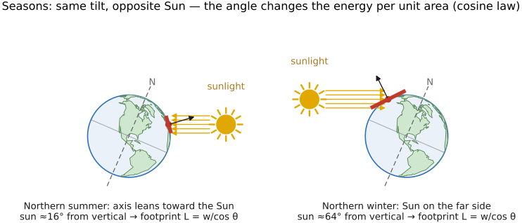
fig-seasons · sidebar — seasons: N. America in summer vs winter (sun angle → energy per area, cosine law) 🟨
fig-polarization-reflection-removal
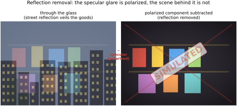
fig-polarization-reflection-removal ·
fig-polarization-dehaze
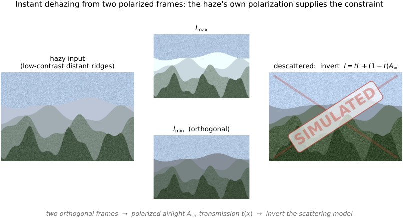
fig-polarization-dehaze ·
fig-polarization-mosaic
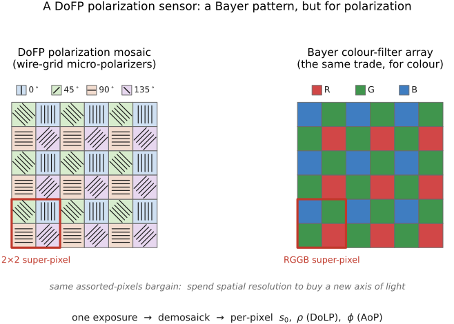
fig-polarization-mosaic ·
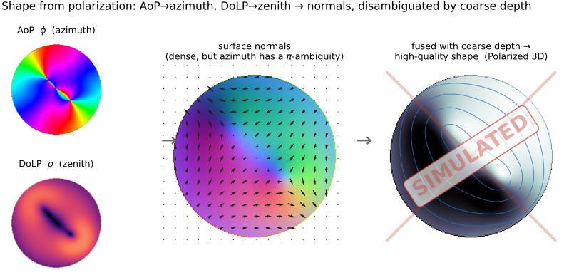
fig-shape-from-polarization
fig-shape-from-polarization ·
💡 **Big lesson (L11.2 · Capture the full set, decide later — polarization axis):** an ordinary camera collapses the light's oscillation orientation at the instant of capture, just as RGB collapses the spectrum. Record a small **stack across polarizer angles** and you can defer questions intensity can't answer — *is this glare or surface?*, *how far through the haze?*, *which way does this facet face?* — to a per-pixel computation afterward. It is the same defer-the-decision move as HDR (exposure), hyperspectral (wavelength) and light fields (aperture), now on the **polarization axis** — and a clean illustration of the plenoptic lesson that the *same* capture-a-stack-and-combine machinery recurs on every axis of light. (→ see Big lesson **L11.2**, [[Big Lessons]].)
equations
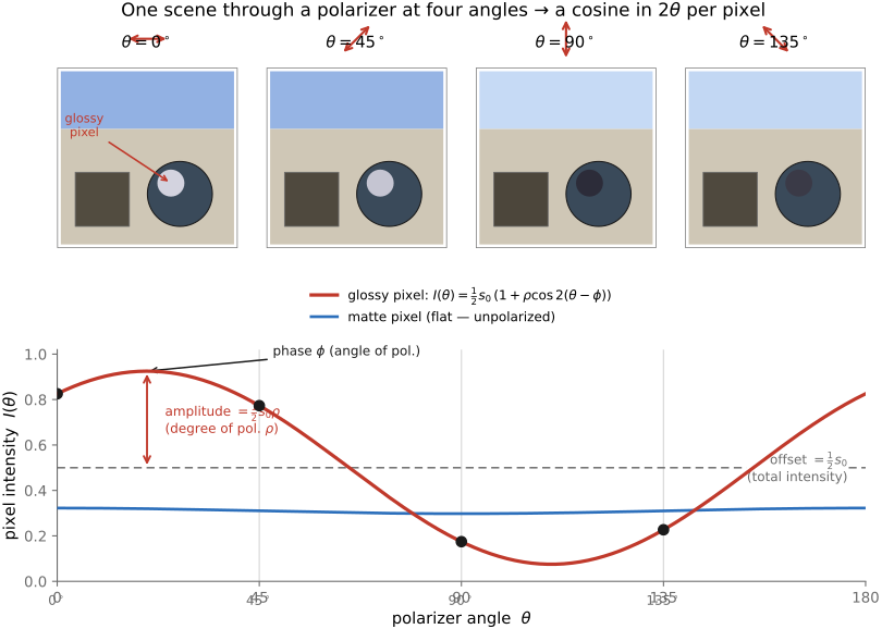
**per-angle intensity (Malus)** $I(\theta)=\tfrac12\,s_0\,\big(1 + \rho\cos(2(\theta-\phi))\big)$ — fit a cosine in $2\theta$ to the measured angles to get total intensity $s_0$, **DoLP** $\rho=\sqrt{s_1^2+s_2^2}/s_0$, **AoP** $\phi=\tfrac12\operatorname{atan2}(s_2,s_1)$
**Stokes (linear)** $s_0=I_0+I_{90}$, $s_1=I_0-I_{90}$, $s_2=I_{45}-I_{135}$
**specular/diffuse split** — the polarized component (varying part of $I(\theta)$) is dominated by **specular/surface** reflection, the unpolarized offset by **diffuse/body** reflection, so $I_\text{diffuse}\approx I_\text{min}$, $I_\text{specular}\approx I_\text{max}-I_\text{min}$
**polarization dehazing** — airlight is partially polarized, so $\hat A_\infty,\
t(x)$ recovered from $I_\text{max},I_\text{min}$ and the airlight DoLP, then invert $I=t\,L+(1-t)A_\infty$.