Computational Photography, an AI-powered Slopendium — 14 Super-resolution and upscaling

▸Part 14 SUPER-RESOLUTION AND UPSCALING⧉

▸14.1 What can super-resolution actually do?⧉

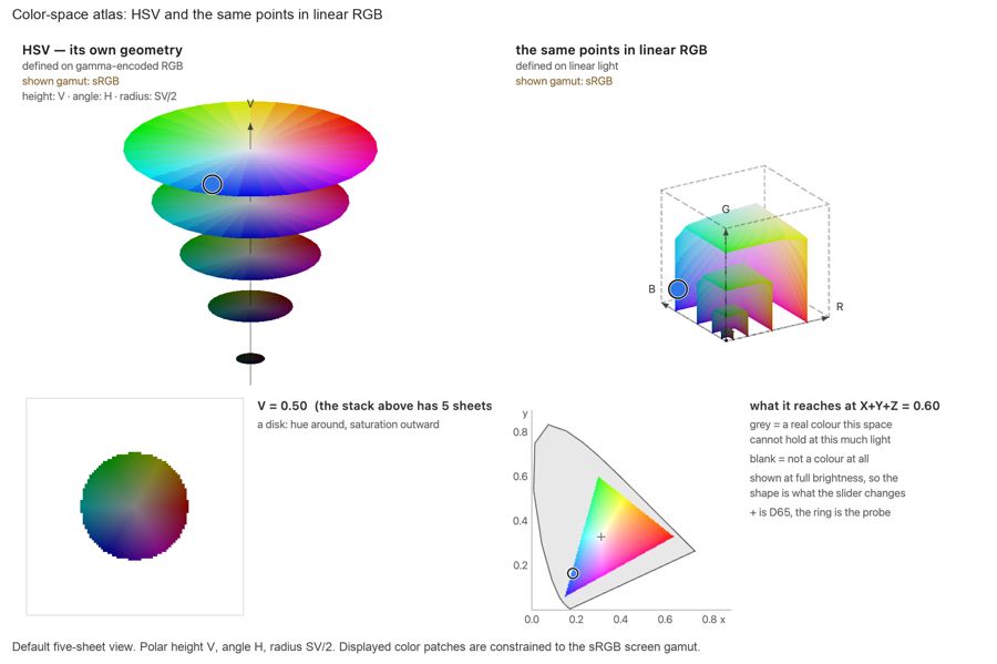
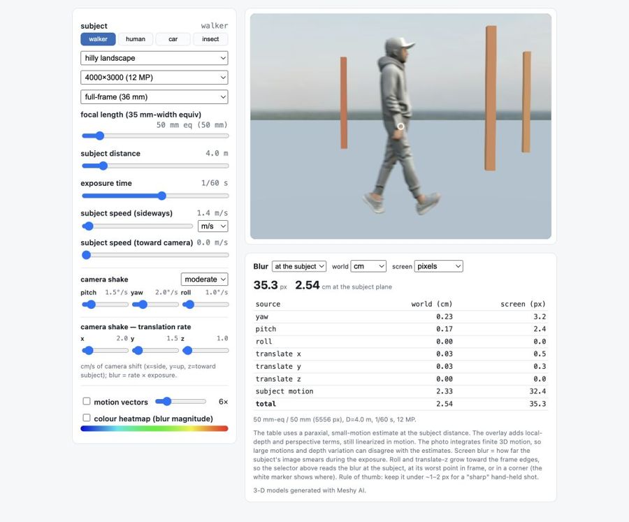
`fig-color-space-atlas` · **interactive** color-space atlas: one space drawn twice, in its own geometry (cube / cone / bi-cone / warped cube) and in a chosen ambient frame (XYZ, LMS, linear RGB, sRGB, Chong, Oklab), from the same lattice, as edges / voxels / one slice; MacAdam ellipses optional; click to read coordinates in both; stripes for colors outside sRGB. Placed at the end of the perceptually-uniform section of **4.6 Advanced color**, where it works as the chapter's capstone: by then HSV/HSL, CIELAB, Oklab and Chong have each been shown alone, and the atlas is about the map between them. URL carries the state (`?space=&ambient=&mode=&axis=&at=&grid=&macadam=&zebra=`). 🟨

`fig-motion-blur-calculator` · live motion-blur calculator: a 3-D scene (walking figure or a car) imaged by a virtual camera, the blur rendered by **temporal supersampling** (many instants across the exposure, averaged). Set resolution / sensor / focal length (35 mm-equiv) / distance / exposure, add camera-shake **rates** in rotation (pitch/yaw/roll) and translation (x/y/z) plus a subject speed; the readout gives the blur at the subject in world (cm/m/in) and screen (px / % width) units, broken down by source. A per-pixel **G-buffer** (depth + subject mask) drives exact motion-vector arrows and a blur-magnitude heatmap: the subject carries its own motion, the background only camera shake. Environment backdrops + car color picker. Static fallback is a screenshot. *3D models generated with Meshy AI.* ✅

equations

the forward model $y = SBx + n$

Nyquist and the folded spectrum.

14.1.1 What the sensor kept and what it folded⧉

14.1.2 The forward model, and why this is an inverse problem⧉

14.1.3 Two operations, one word⧉

14.1.4 What a resolution number means once a prior is involved⧉

▸14.2 Multi-frame super-resolution⧉

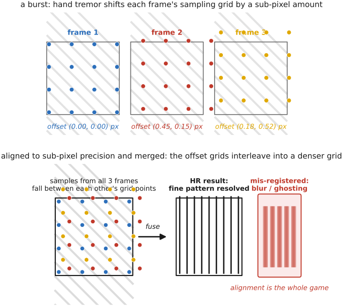
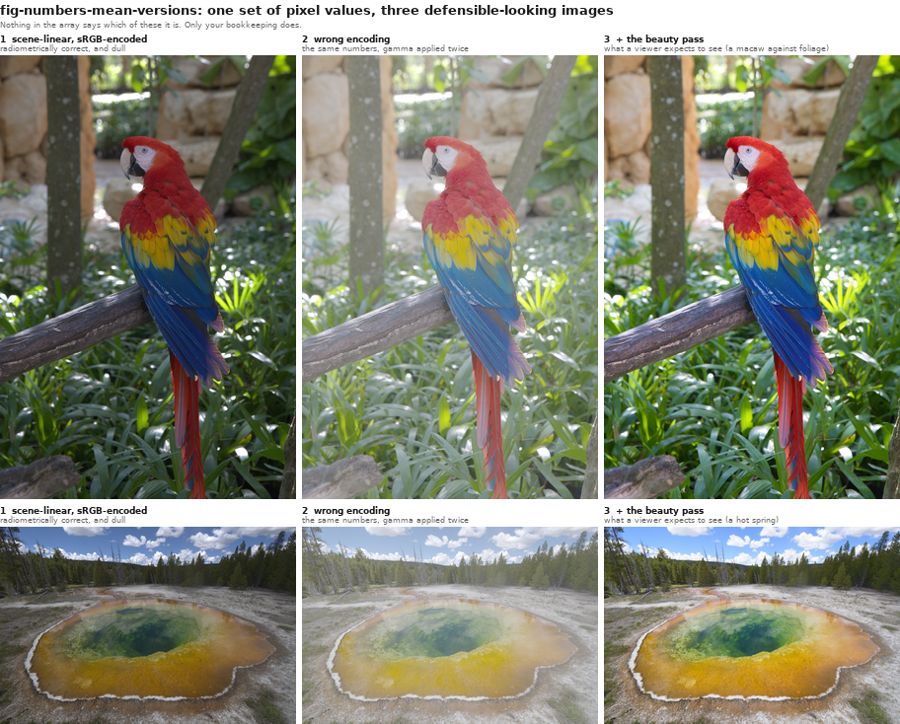
`fig-burst-subpixel` · hand-jitter across a burst lands samples between the LR grid points; merging the sub-pixel-shifted frames fills the HR grid 🟨

`fig-numbers-mean-versions` · one set of raw-DNG pixel values rendered three plausible ways — scene-linear→sRGB (dull but correct) · the same numbers mis-encoded (double gamma) · + beauty pass (what a viewer expects); makes "numbers are meaningless without their encoding" concrete (Image representation → what the numbers mean, BASIC) ✅

equations

the multi-frame forward model with a per-frame warp $y_k = S B W_k x + n_k$

the back-projection update.

14.2.1 Sub-pixel shifts are extra samples⧉

14.2.2 The classical formulations⧉

14.2.3 Registration is the hard part⧉

14.2.4 What actually ships⧉

14.2.5 The gain, and where it stops⧉

▸14.3 Learned burst methods⧉

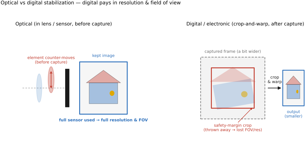
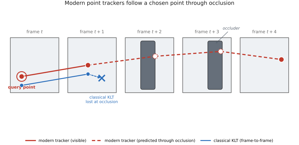
`fig-digital-vs-optical-stab` · optical (in lens/sensor, before capture, full resolution & FOV) vs digital/electronic IS (crop-and-warp in software after capture): the EIS safety-margin crop + warp costing resolution/field of view vs the optical in-lens/sensor correction ✅

`fig-modern-point-trackers` · long-range point tracking (TAP/PIPs/CoTracker) — a query point followed across frames as one trajectory, persisting through occlusion (dashed), where classical KLT loses it ✅

equations

the permutation-invariant form, a per-frame encoder, a symmetric pooling over frames, and a decoder, so the output depends on the SET of frames and not their order.

14.3.1 Aligning in features, merging by attention⧉

14.3.2 A burst is a set, not a sequence⧉

14.3.3 Where the training data comes from⧉

14.3.4 What a learned merge does that a kernel cannot, and what it costs⧉

▸14.4 Single-image super-resolution: classical methods⧉

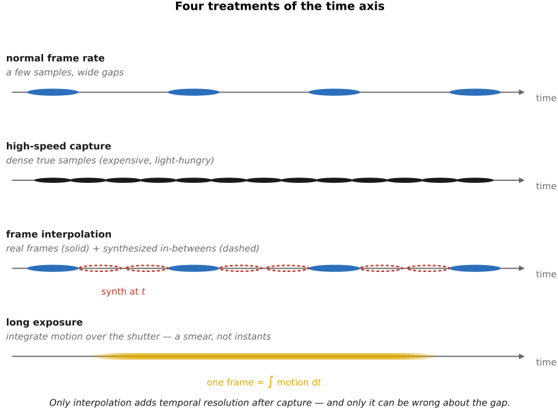
`fig-slowmo-axis` · four ways to treat the time axis on a shared timeline — normal capture (sparse), high-speed (dense true samples), interpolation (sparse reals with synthesized in-betweens), and long-exposure blur (the integral); only interpolation adds resolution after capture and can be wrong 🟨

equations

the sparse-coding formulation with coupled dictionaries.

14.4.1 Interpolation, and what it actually assumes⧉

14.4.2 Example-based super-resolution⧉

14.4.3 Neighbor embedding and the manifold assumption⧉

14.4.4 Sparse coding and dictionary learning⧉

14.4.5 RAISR: a bank of learned filters, chosen by hashing⧉

14.4.6 The image as its own database⧉

▸14.5 Single-image super-resolution: deep learning⧉

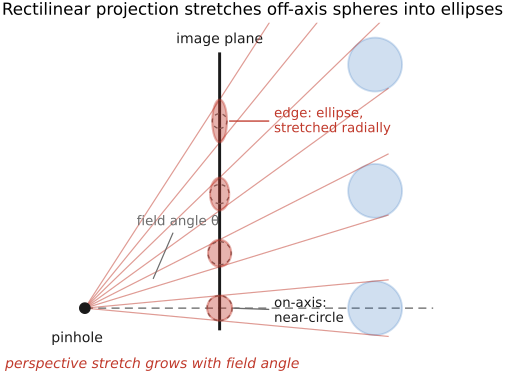
`fig-wide-angle-perspective-distortion` · wide-angle perspective distortion: off-axis spheres image as radially-stretched ellipses (flat-sensor geometry), and faces near a wide frame's edge are widened — not a lens flaw; forward-ref to correction (Pinhole image formation) ✅

14.5.1 The architectural line⧉

14.5.2 Where the upsampling goes⧉

14.5.3 The ceiling, and what it was made of⧉

14.5.4 What these networks do and do not learn⧉

▸14.6 The perception-distortion tradeoff and perceptual super-resolution⧉

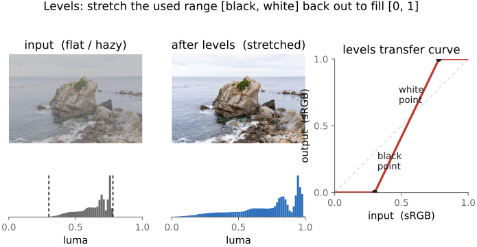
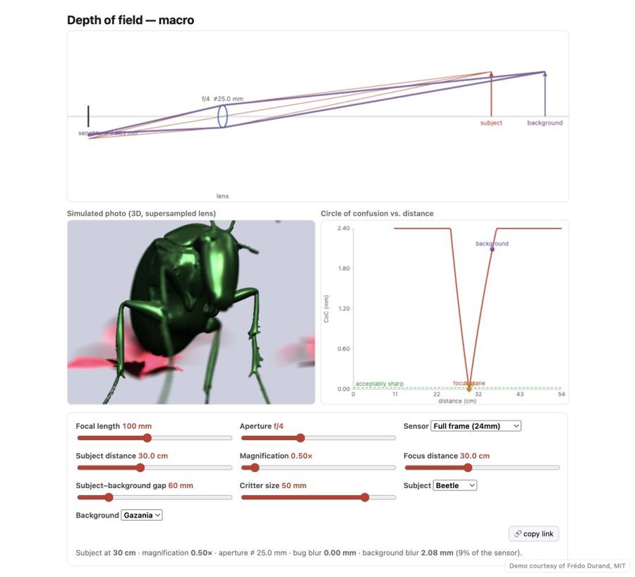
`fig-point-op-levels` · levels on a real (flat/hazy) photo: bunched-up luma histogram stretched out to fill [0,1] by setting a black point and a white point — input + after + transfer curve with the clip-and-stretch anchors and the two histograms (Point operations → Black point, white point, and levels, BASIC) ✅

`fig-depth-of-field-sim` · live macro depth-of-field simulator (web edition): a to-scale thin-lens diagram + a 3D photo (aperture-supersampled bokeh) + a circle-of-confusion plot all sharing one optics model; subject dropdown (Meshy beetle / bee / ladybug) over a flower background, focus landing on the front of the face so the body and antennae blur; static fallback is a screenshot. *Bug & flower 3D models generated with Meshy AI.* ✅

14.6.1 The tradeoff, stated⧉

14.6.2 Buying perceptual quality: perceptual losses and adversaries⧉

14.6.3 Measuring on both axes⧉

14.6.4 The hallucination problem⧉

▸14.7 Generative super-resolution⧉

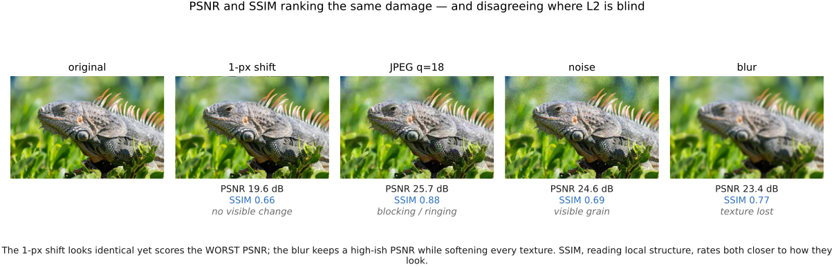
`fig-metric-degradation-gallery` · one clean photo vs four degradations (1-px shift, low-q JPEG, noise, blur), each labeled with PSNR + SSIM — PSNR and SSIM mostly agree but disagree where L2 is blind (shift scores worst PSNR yet looks identical; blur keeps high PSNR yet softens texture) (Image metrics, BASIC) ✅

14.7.1 Conditional generation⧉

14.7.2 Sampling against averaging⧉

14.7.3 Consistency, faithfulness, and what to report⧉

14.7.4 The circle closes⧉

▸14.8 Reference-based and domain-specific super-resolution⧉

14.8.1 Reference-based super-resolution⧉

14.8.2 Face and text restoration⧉

14.8.3 One model, any scale⧉

14.8.4 Learning from the test image alone⧉

14.8.5 The ordering, stated⧉

14.9.1 The real degradation chain⧉

14.9.2 Degradation modeling: the fix was data⧉

14.9.3 Estimating the degradation instead of covering it⧉

14.9.4 Real paired data, and the gap that remains⧉

▸14.10 Video super-resolution and practical systems⧉

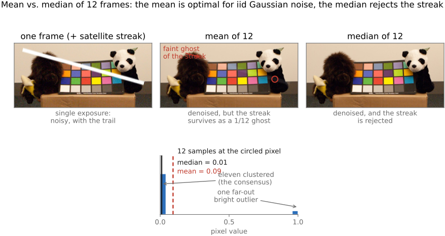
`fig-mean-vs-median-stack` · plain-mean stack (residual ghost streak from one outlier frame) vs median / sigma-clip stack (streak rejected) of the same frames, with the per-pixel sample distribution inset ✅

14.10.1 Temporal consistency is the new constraint⧉

14.10.2 Using the neighbors⧉

14.10.3 Hybrid space-time super-resolution⧉

14.10.4 What is deployed⧉

14.10.5 What super-resolution actually delivers⧉

14.11 Super-resolution TLDR⧉