3.13 Auto-exposure and auto white balance⧉
A camera makes two guesses about light on every shot, and both are under-determined — they must recover intent from pixels that confound the answer. Auto-exposure (AE) decides how much light to collect; auto white balance (AWB) decides what color the light was so it can be divided out. Neither has a labelled ground truth in the frame, so each leans on assumptions, and the history of both is the story of those assumptions getting smarter: a flat average, then a zone/pattern model, then a learned one.
3.13.1 Auto-exposure: metering⧉
Before the shutter even opens, the camera must choose aperture, shutter, and ISO so the scene lands at a sensible brightness — the metering problem. The reference is the middle-grey target (≈18% reflectance) from the exposure discussion in Photography and camera 101: the meter tries to place the scene's representative tone there. The catch is exactly the one white balance hits below — which pixels are representative? — and metering modes are a ladder of ever-smarter answers.
Average and center-weighted metering. The simplest meter averages the whole frame to one number and exposes so that average is middle grey. It is fooled by anything that is not average: a bright sky pulls the average up, so the meter under-exposes and the foreground falls into shadow (the classic backlit-subject silhouette); a snow field reads too bright and is rendered a dingy grey. Center-weighted metering improves the guess by weighting the middle of the frame most, on the assumption that the subject is usually near the center.
Matrix / evaluative / pattern metering. Modern cameras divide the frame into a grid of zones and combine them intelligently rather than flatly. They measure each zone's brightness, the contrast between zones, which zone holds the focus point, and sometimes color, and feed those into a model — historically a lookup against a database of tens of thousands of reference scenes. Nikon's 3D Color Matrix metering folds in color and the distance the lens reports (hence "3D"); Canon's evaluative and others are cousins. The model recognizes patterns like "bright top zone, darker bottom, subject in focus near the center → backlit landscape" and biases the exposure to protect the subject. This pattern/evaluative metering is the default on every modern camera.
Spot metering is the opposite extreme: meter one small zone and place that tone at middle grey. It hands the photographer exact control over which tone is anchored — the basis of Ansel Adams's Zone System — at the cost of having to choose wisely.

Learned metering. The newest cameras and phones replace the hand-built zone model with a machine-learned one: a small network looks at a downsampled frame (often plus a semantic segmentation — sky, face, backlight) and predicts the exposure a good photographer would pick, trained on large sets of human-rated images. Phones go further and choose exposure jointly with their burst / HDR pipeline, deliberately under-exposing each frame to protect highlights and then recovering the shadows by stacking (→ multiple-exposure imaging) — leaning on the affine-and-truncated noise model from the noise chapter to know how far the shadows can be pushed. Auto-exposure has thus traveled the same arc we are about to see for auto white balance: one hand-coded statistic → a multi-zone pattern model → a learned estimator, all guessing intent from pixels.
Auto white balance is the color twin of this exposure guess, and it climbs the very same ladder.
3.13.2 white balance and color constancy⧉
We arrive at the camera's hardest color guess. The light that reaches the sensor is the product of the illuminant spectrum and the surface reflectance — so a white shirt under tungsten light sends warm, orange-ish light to the sensor, and the very same shirt under open shade sends cool, bluish light. Yet to a human the shirt looks white under both, because the visual system discounts the illuminant — the color constancy of the perception chapter. A camera has no such automatic constancy; it must estimate the illuminant and divide it out, and that operation is white balance (Figure 3.13.2).
The standard model is beautifully simple. Von Kries adaptation says: correct each color channel by an independent gain,
a diagonal $3 \times 3$ transform (Figure 3.13.3). The gains are chosen so that a known neutral in the scene comes out neutral ($R' = G' = B'$). This is the same diagonal-adaptation idea as the Bradford transform in color management, and it is the spectral-domain stand-in for what the cones do biologically (Land and McCann's Retinex, 1971, is the influential model of how the visual system might compute it). A general $3 \times 3$ matrix can do a little better than the pure diagonal when channels interact, but the diagonal von Kries gain is the workhorse.

One subtlety dictates where in the pipeline this correction belongs. White balance is a per-channel multiply, and a scaling commutes with a linear map but not with a non-linear one. Apply the same gains $k_R, k_G, k_B$ to linear-light values and you simply rescale the channels, as intended; apply them instead to gamma- or tone-curve-encoded (non-linear) values and the result is wrong — the gains no longer merely neutralize the cast but also shift hue and change apparent saturation (Figure 3.13.4). The reason is exactly the additive-vs-multiplicative lesson from the encoding section: a multiply is only faithful in the space where the arithmetic is linear. So white balance, like exposure (another multiply-in-linear-light), belongs early, in the linear part of the pipeline, before the gamma curve is applied — get the order wrong and you tint the very colors you were trying to correct.

3.13.3 Automatic white balance⧉
In practice the camera has no labelled neutral patch, so it must guess the illuminant from the image itself — automatic white balance (AWB). The classic assumptions are statistical. Grey-world assumes the scene averages to grey, so the channel gains are
scaling each channel so the means agree (Figure 3.13.5). The bright-pixel (white-patch) assumption instead takes the brightest pixels to be a white highlight reflecting the illuminant directly, and balances on those. Both fail in predictable ways — grey-world tips on a scene dominated by one color (a forest, a red wall), bright-pixel tips on a colored specular highlight.

Modern cameras go well beyond these. A common middle ground is to regress the illuminant from image statistics with a learned $3 \times 3$ correction, and the current best methods are machine-learned color constancy — a small network or a learned histogram model (Barron's Fast Fourier Color Constancy, 2017, recasts the estimate as a convolution over a log-chroma histogram). These learn the priors that grey-world and bright-pixel only crudely assume, but they are still solving the same under-determined problem: recover two numbers (the illuminant's chromaticity) from an image that confounds light and surface.
The key reframing is to stop thinking of the image as a picture and start thinking of it as a histogram of log-chroma: bin every pixel by the ratios of its channels (how red-to-green, how blue-to-green it is), and a global change of illuminant simply translates that whole histogram rigidly across the log-chroma plane. Estimating the illuminant is then nothing but finding where the histogram has been shifted to — a localization problem — which a learned filter can solve as a single convolution, made fast by doing it in the Fourier domain. The figures below walk through the method.


Color-constancy sets with ColorChecker ground-truth illuminant; lead with NUS (8 cameras), cite Gehler-Shi as the classic baseline. <https://www2.cs.sfu.ca/~color/data/shi_gehler/> · <https://cvil.eecs.yorku.ca/projects/public_html/illuminant/illuminant.html>. See the Datasets appendix.
Skin is the colour cameras are quietly tuned around, for two reasons. First, faces are the most common and most scrutinised subject, and skin is a memory colour — we have a strong prior for what it should look like — so modern metering and white balance are biased to render it well: face detection feeds both the meter and the AWB so that the person, not the average scene, lands at a sensible exposure and a believable warmth. Second, and less happily, that tuning carries a history of bias. Colour film, and later automatic exposure and white balance, were calibrated against the Shirley card — a reference photo of a light-skinned woman — so the defaults were fit to light skin and rendered darker skin poorly (under-exposed, with the wrong cast), a bias that persists wherever metering, white balance, and face detection inherit those defaults. The obligation is concrete: design and test exposure and white balance across the full range of skin tones, not just the historical reference. We take this up as an ethics question — the Shirley card, fairness in capture — in Ethics of computational photography.
3.13.4 The limits of white balance, and CRI⧉
White balance is one global guess, and two situations defeat it no matter how clever the estimator — the second of which forces us to measure the quality of the light itself, its color rendering index (CRI). The first is mixed illumination: a single per-channel gain cannot simultaneously fix a face lit warm by a lamp and cool by a window, because the right correction differs across the frame (Figure 3.13.12). Doing it properly needs per-region or multi-light white balance, which we take up in the advanced material (Hsu et al.). The second is metameric failure of the illuminant. White balance can only rescale channels; it cannot resurrect color information the light never delivered. A light with a spiky, gap-ridden spectrum — a cheap fluorescent tube or a low-quality LED — simply fails to illuminate certain wavelengths, so reflectances that differ only in those bands collapse to the same camera response and no gain can pull them apart.
This is exactly the regime Hsu and colleagues set out to crack: not a cleverer global gain, but a per-pixel estimate of which light is doing the lighting, and then a different correction at every point. Their three figures below carry the argument from the failure to the fix.


The quality of a light source is quantified by its CRI (color rendering index): how faithfully a source renders a set of test colors compared with a reference illuminant of the same correlated color temperature. A perfect incandescent or daylight source scores $100$; a spiky fluorescent or cheap LED may score in the $50$s, mis-rendering whole families of color even after white balance (Figure 3.13.16). High CRI is why good studios and museums pay for their lights, and why two prints can match under daylight yet diverge under store fluorescents — illuminant metamerism made expensive.

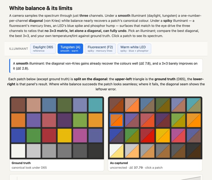
It is worth playing with this limit, because the failure is sharper than a static figure can show. The interactive demo below renders a ColorChecker from spectra: pick an illuminant — smooth daylight, a warm tungsten, or a spiky fluorescent or LED — and watch the captured chart, each patch's resulting spectrum (reflectance × illuminant), and the best white balance attainable two ways: a diagonal (von Kries) correction and a full $3\times3$ matrix, each fit by least squares against the D65 ground truth, with its residual error printed (Figure 3.13.17). Under a smooth light the diagonal nearly recovers the truth and the $3\times3$ closes the rest. Under a spiky light the residual will not go to zero — not for the diagonal, and not even for the full $3\times3$ — because once the illuminant fails to deliver whole bands of the spectrum, different reflectances collapse to the same three camera numbers and no linear map can pull them back apart. The temperature/tint sliders let you try to white-balance by hand, and you will find you can never match the ground truth on a bad light: a manual correction is only a diagonal, and a diagonal is the weakest of the corrections that already cannot win.