• **the observation**, before any math: point a tripod-mounted camera at a static, evenly-lit grey patch and shoot a burst. Each pixel *should* read one constant value; instead it **fluctuates** frame to frame, and across the patch (it should be flat) it's grainy. Two faces of the same thing — noise as **fluctuation over time** and **fluctuation over space when the answer should be constant**. [`fig-averaging-N-frames`]

• **the naive algorithm** is a one-liner: sum the frames, divide by $N$.

```

mean = zeros_like(imSeq[0])

for im in imSeq: mean += im

mean /= len(imSeq)

```

Visibly, 1 → 3 → 5 → 45 frames: the grey patch's histogram tightens, dark areas clean up. *Why* — and *how fast*? [`fig-averaging-N-frames`]

• **the model** (the load-bearing assumption): each pixel's value in frame $i$ is the **true signal plus noise**, $X_i = \mu + n_i$, where the noise is **zero-mean** ($\mathbb{E}[n_i]=0$ — averaging is only honest if the noise has no DC offset) and **independent** across frames (frame $i$'s noise tells you nothing about frame $j$'s — true for shot & read noise, *false* for fixed-pattern noise; flag this now, fix it in *Calibration*). Each has variance $\operatorname{Var}[n_i]=\sigma^2$.

• **the two tools** (state them as the reusable algebra): for a random variable, scaling squares the variance, $\operatorname{Var}[kX]=k^2\operatorname{Var}[X]$; and for **independent** variables, **variance of the sum is the sum of variances**, $\operatorname{Var}[\sum_i X_i]=\sum_i\operatorname{Var}[X_i]$ (independence is what kills the cross terms / covariance). [`fig-iid-variance-adds`]

• **the derivation** (two lines): the average is $\bar X=\tfrac1N\sum_i X_i$. Its **mean is the true value** — $\mathbb{E}[\bar X]=\tfrac1N\sum_i\mathbb{E}[X_i]=\mu$ — so averaging is **unbiased**: it doesn't distort the signal. Its **variance**: pull out the $\tfrac1N$ (squares, by the first rule), then add (by independence):

$$\operatorname{Var}[\bar X]=\frac{1}{N^2}\operatorname{Var}\Big[\sum_i X_i\Big]=\frac{1}{N^2}\cdot N\sigma^2=\frac{\sigma^2}{N}.$$

Take the square root for the human-readable number: $\sigma_{\bar X}=\sigma/\sqrt N$.

• 💡 **the punchline — the $1/\sqrt N$ law** (see the big-lesson box above): **variance drops as $1/N$, std as $1/\sqrt N$.** This is the chapter's whole quantitative content. Its sting is the diminishing return: $4\times$ the frames for $1\times$ less noise (one stop); 100 frames buys a $10\times$ cleaner image, not 100×. In SNR terms, $+10\log_{10}N$ dB — about **3 dB per doubling**. [`fig-sqrtN-curve`]

• **estimating the noise itself** (aside, for the analysis pipeline): from the same stack you can *measure* $\sigma^2$ per pixel — but divide by $N-1$, not $N$ (**Bessel's correction**), because you used the same samples to estimate the mean, which correlates the residuals and otherwise *under*-estimates the variance. The coin-flip-with-$N{=}2$ example makes this concrete: the $N$ estimator averages to half the true variance; the $N{-}1$ estimator is unbiased.

• **what it confirms about the sensor** (callback to the noise part): map the measured $\sigma$ across a real scene and it tracks the noise sources — more noise (numerically) in **bright** areas (shot noise $\propto\sqrt{\#\text{photons}}$), yet **better SNR** there; the log-SNR image "looks like the photo." Averaging lowers the floor uniformly; it does not change *which* source dominates where.

• **the failure of the mean**: the derivation assumed *clean* IID noise. A real stack has **outliers** — a satellite or plane streaks one frame, a cosmic ray spikes a pixel, someone walks through. The mean is **not robust**: a single wild value drags the average, leaving a faint **ghost trail** exactly where the outlier was. [`fig-mean-vs-median-stack`]

• **median**: take the per-pixel **median** across the stack instead of the mean. One streaked frame is just an extreme value the median ignores → the streak vanishes. Cost: the median is **noisier than the mean** for clean Gaussian data (its variance is $\approx\!1.57\times$ larger, so you lose roughly a third of your $\sqrt N$ benefit) — robustness isn't free.

• **sigma-clipping** (the practical compromise, the astro/stacking default): iterate — compute per-pixel mean and std, **reject** samples more than $k\sigma$ (say $2$–$3\sigma$) from the mean, recompute on the survivors. You get the mean's **efficiency** on the inliers *and* the median's **rejection** of outliers. This is what RegiStax / DeepSkyStacker do under "kappa-sigma" or "winsorized" stacking.

• **the design choice to surface**: this is the same *reject-or-average* decision as edge-preserving filtering (**L4** — use a difference to decide who belongs together), now applied **across frames** instead of across space: a sample too far from its peers is treated as not-belonging. Plain mean = trust everyone; median/sigma-clip = trust the consensus.

• **forward-ref**: the same robust-combine logic reappears as **de-ghosting** in HDR merging and panoramas (reject pixels that disagree because something *moved*), and as the **robust merge** in burst SR ([[Super-resolution and image priors]]).

• **the limit of averaging** (callback to the model): the $1/\sqrt N$ law only kills **zero-mean, independent** noise. Two things break that assumption and survive any amount of averaging — **fixed-pattern** offsets (the *same* error every frame: hot pixels, amp glow, per-pixel dark current, vignetting, dust shadows) and **clipping** (a non-linearity that biases the mean). These need to be *removed*, not averaged. [`fig-calibration-triad`]

• **the calibration triad** — each frame is the inverse of one degradation:

• **bias / offset**: shoot the shortest possible exposure with the lens capped → captures the read-out **electronic offset** (and the deliberate offset many cameras add so noise stays *zero-mean* — see clipping below). **Subtract** it.

• **darks**: shoot capped frames at the **same exposure time and temperature** as your lights → captures **dark current** (thermal charge that accumulates per second) and **hot pixels**. **Subtract** them. *This is why astro cameras are **cooled and temperature-regulated*** — dark current roughly doubles every 6–8 °C, and a *repeatable* temperature makes the dark frame actually match the light frame (callback to FUNDAMENTALS — cooled cameras, **L15** lower floor).

• **flats**: shoot an evenly-lit blank field → captures the **multiplicative** response variation — **vignetting** (corners darker) and **dust** shadows. **Divide** by it (normalised).

• in one expression: $X_\text{cal}=\dfrac{X_\text{light}-X_\text{dark}}{X_\text{flat}-X_\text{bias}}$ — subtract the **additive** fixed-pattern terms, divide out the **multiplicative** ones. (And you average *many* of each calibration frame too, so they don't re-inject noise — $1/\sqrt N$ all the way down.)

• **the clipping bias** (a subtle one worth a figure): the sensor **clamps at 0 and at max**, so in deep shadows the noise is *not* zero-mean — the below-zero excursions are cut off, leaving only the positive ones. Averaging then pulls a true-black region **too bright**. The fix is a **deliberate positive offset** (Canon's trick) added before read-out so the full noise distribution stays above 0 and *stays zero-mean*; subtract it back in calibration. [`fig-clipping-bias`]

• **dithering** (the trick that *converts* fixed-pattern into averageable noise): deliberately **nudge the framing** a pixel or two between frames. After re-alignment, any residual fixed-pattern error lands on a *different* part of the sky each frame, so it becomes effectively random across the registered stack — and *then* averaging/clipping can remove it. (This is also why burst SR's hand-tremor is a feature, not a bug — [[Super-resolution and image priors]].)

• the purest use of "average to denoise": a faint nebula/galaxy buried in noise and light pollution → shoot **many long "subs"**, **align** them (the sky rotates — cross-ref [[#Image alignment]] below), and **average** → signal stays while noise falls as **1/√N**, pulling structure out of near-nothing. This is the $1/\sqrt N$ law pushed to its physical limit: hours of total integration (hundreds of subs) to lift a galaxy that is *invisible* in any single frame. [`fig-astro-stack-reveal`]

• **calibration frames** matter as much as the lights: subtract **darks** (dark current + hot pixels — why cooled astro cameras regulate temperature), divide by **flats** (vignetting + dust), remove **bias/offset** — the fixed-pattern terms of the noise chapter, taken out by calibration (see *Calibration frames* above — astro is where the triad is non-negotiable).

• **robust combine, not a plain mean**: per-pixel **sigma-clipping / median** across the stack rejects satellites, planes, and cosmic rays; **dithering** (nudging the framing between subs) turns fixed-pattern residue into something averaging *can* remove (see *robust combination* and *dithering* above). [`fig-mean-vs-median-stack`]

• the budget: read noise per sub favors **fewer, longer** subs; saturation, tracking error, and clipping favor **more, shorter** ones — the same exposure trade-off, astro edition (cross-ref [[Noise, signal-to-noise ratio and dynamic range]], ETTR). Quantitatively: once each sub's signal is well **above the read-noise floor**, lengthening subs no longer helps the $\sqrt N$ math — but it reduces the *number* of read-noise events, so when read noise is significant (light-polluted or narrowband), **fewer-longer** wins; when tracking is shaky or stars saturate, **more-shorter** wins. [`fig-sub-length-tradeoff`]

• cross-ref: **cooled cameras** (FUNDAMENTALS *Cameras beyond photography*); **lucky imaging** for planetary (Big data — pick the *sharpest* frames rather than averaging all, when atmospheric seeing dominates); the **astro hub** (Adjacent fields). Note the contrast with planetary lucky imaging: deep-sky *averages everything* to beat read/shot noise; planetary *selects the best few percent* to beat atmospheric blur — same burst, opposite combine rule.

• **the precondition**, made vivid: take a hand-held burst and average it *without* aligning → you don't get a cleaner image, you get a **blurry double**. The $1/\sqrt N$ benefit only materialises once the frames agree pixel-for-pixel; alignment is what *earns* it. [`fig-align-before-average`]

• **the two failure scales**: a **sub-pixel** misalignment loses fine detail (the average smears across the offset — a soft low-pass); a **whole-pixel-or-more** misalignment **ghosts** (edges appear twice). In astro the driver is unavoidable — the **sky rotates** through the exposure, so without per-sub alignment the stars trail and the stack is mush.

• **the reframe**: alignment is itself an **inverse problem / optimization** — find the transform $T$ that makes $I_2(T\!\cdot)$ match $I_1$, i.e. $\hat T=\arg\min_T\sum_x\big(I_1(x)-I_2(Tx)\big)^2$. Everything below is *which family of $T$* (translation, homography, dense flow) and *how you search it*.

• **the simplest model — pure translation**: for a tight burst, frame-to-frame motion is well-approximated by a 2-D **shift** $(dx,dy)$. Try **all shifts** within $\pm\,$maxOffset and keep the best-scoring one. (This is literally a pset: brute force over a shift window.)

• **the score — SSD**: sum of squared differences, $\mathrm{SSD}(dx,dy)=\sum_{x,y}\big(I_1(x,y)-I_2(x{+}dx,y{+}dy)\big)^2$ — small when the frames agree. Plot it over the shift window and you get a **basin with a clear minimum** at the true shift. [`fig-ssd-search-surface`]

• *pseudocode*: the brute-force aligner as a double loop over the shift window — score each candidate by SSD, keep the argmin.

• **when SSD lies — NCC**: SSD assumes **brightness constancy** (same exposure/illumination). Across an HDR bracket or with a brightness drift, that's false and SSD breaks. **Normalised cross-correlation** is invariant to a per-frame **gain and offset** — subtract each patch's mean, divide by its std, correlate: $\mathrm{NCC}=\dfrac{\sum (I_1-\bar I_1)(I_2-\bar I_2)}{\sqrt{\sum(I_1-\bar I_1)^2}\,\sqrt{\sum(I_2-\bar I_2)^2}}$, **maximised** at the true alignment. Use SSD for same-exposure bursts, NCC (or align in a normalised/gradient domain) when brightness changes between frames.

• **debugging / hand-checkable input**: align a synthetic image to a copy of itself **shifted by 1–2 px** — the alignment score (e.g. SSD of the difference) must be **smallest at the true shift**; validate the search this way before trusting real data. Concretely: shift a known image by $(+2,0)$, run the search, and confirm the score map's minimum sits *exactly* at $(+2,0)$. If it doesn't, your indexing/sign/interpolation is wrong — and you'll never catch it on noisy real frames. This shifted-copy test is the cheapest, most reliable unit test an aligner has. [`fig-shifted-copy-debug`]

• **sub-pixel refinement** (forward-ref): integer-shift search gets you close; fit a parabola to the SSD basin (or upsample) for **sub-pixel** accuracy — which is exactly the precision burst **super-resolution** depends on ([[Super-resolution and image priors]]). Shifting by a fractional pixel means **interpolation** (bilinear/bicubic — BASIC Resampling).

• **the idea** (and the lesson): a **pure shift** is, in Fourier, just a **phase ramp** — the magnitudes are unchanged, only the phases tilt: $I_2(x)=I_1(x-d)\Leftrightarrow\hat I_2(\omega)=\hat I_1(\omega)e^{-i\omega\cdot d}$ (the **shift theorem**). So the *entire* translation lives in the phase. 💡 **Big lesson (L5 · diagonalize when you can):** convolution and correlation are **diagonal in Fourier** — instead of an $O(\text{window}^2)$ search over shifts, one FFT pair recovers the global shift directly. (→ see Big lesson **L5**, first placed in BASIC — [[Linearity, Fourier, Aliasing and deblurring]]; here it turns brute-force search into a single transform.)

• **the algorithm** — phase correlation (Kuglin & Hines 1975): form the **normalised cross-power spectrum** $R(\omega)=\dfrac{\hat I_1\,\overline{\hat I_2}}{|\hat I_1\,\overline{\hat I_2}|}=e^{i\omega\cdot d}$ (normalising to *unit magnitude* keeps only the phase — robust to brightness and to dominant low-frequency content). Its inverse transform $\mathcal F^{-1}\{R\}$ is a **single sharp delta at the shift $d$** — read off the peak location. [`fig-phase-correlation-spike`]

• **why it's nice**: global, fast ($O(n\log n)$), and the delta's **sharpness/height** doubles as a confidence measure. Extends (log-polar — Reddy & Chatterji 1996) to recover **rotation and scale** as shifts in a transformed domain.

• **its limits** (be honest): it assumes a **single global shift** over the whole frame — it can't handle parallax, scene motion, or a per-region warp. Those need a richer transform (homography → panorama chapter) or **per-pixel** motion (optical flow → video).

• **the two problems brute force has**: large motions blow up the search window (cost), and a raw SSD surface can have **local minima** (texture/aliasing) that trap a naive search.

• **the fix — multiscale**: build an **image pyramid** (cross-ref [[Linear pyramids and wavelets]]) and align **coarse-to-fine**. At the coarsest (tiny, blurred) level a *small* shift covers a *large* real motion and the score surface is smooth (no local minima) → get a cheap rough estimate; **propagate it down**, refining at each finer level with only a tiny local search. [`fig-coarse-to-fine-pyramid`]

• **why it works** (frequency view, **L5/L16**): the coarse level keeps only **low frequencies**, whose SSD basin is wide and unimodal; finer levels add the high-frequency detail that sharpens the estimate but would otherwise create false minima. Prefiltering on the way down the pyramid is the same **L16** "blur before you decimate" discipline.

• **in production**: HDR+ (Hasinoff 2016) aligns burst frames this way — a **tiled, coarse-to-fine** search per tile, then a robust merge — handling both global hand motion and local scene motion at once.

• **the hand-off to video**: replace "one transform per frame" with "**one motion vector per pixel**" and coarse-to-fine matching becomes **optical flow**; constrain $T$ to a homography and it becomes **stabilization / panorama**. The alignment machinery here is the entry point to [[Slopendium/09 Motion, warping, and video|Motion, warping, and video]] — *this chapter links forward there.*

• **the gap, stated in numbers**: real scenes span **10 to 12 orders of magnitude** of illumination (the eye adapts from $\sim 10^{-6}$ to $10^{6}$ cd/m²; a single indoor-with-window scene is routinely $1{:}100{,}000$). A negative or sensor records only **2–3 orders** in one shot; a print or display shows even less — typically $1{:}20$ to $1{:}50$, at best $\sim 1{:}500$. *Two distinct problems fall out:* **(1) record** the information (a single capture can't), and **(2) display** it (the medium can't show it even once recorded). This chapter is problem (1) — **recording** via merge. Problem (2), **tone reproduction**, is forward/elsewhere. [`fig-dr-clip-vs-noise`]

• **why one exposure fails — the two walls** (this *is* **L15**): turn exposure up and the **highlights clip** — any radiance past the photosite's full-well capacity saturates to the max value, all detail above it collapses to white. Turn exposure down and the **shadows drown** — the signal sinks below the **read-noise floor**, and brightening them in post just amplifies noise. The window between the two walls is the **single-shot dynamic range**; a high-DR scene doesn't fit. [`fig-dr-clip-vs-noise`]

• **the formation model** (carry it through the whole chapter): scene radiance $L(x,y)$ reaches a photosite, is scaled by an **exposure factor** $k_i$ (set by shutter, aperture, ISO), has **noise** added, and **clips** above the well capacity: $I_i(x,y)=\mathrm{clip}\big(k_i\,L(x,y)+n\big)$. Everything below is *invert this*: estimate the single $L$ from the several clipped, noisy $I_i$.

• **the resolution — bracket and merge** (this *is* **L14**): shoot $N$ exposures that **sequentially measure different segments of the range** — a short one keeps the highlights, a long one digs out the shadows. Each $I_i$ is reliable only over a *band* of radiance (above its noise, below its clip); slide the band with $t_i$ and the bands tile the whole scene range. Merge the reliable parts into one floating-point radiance map. [`fig-exposure-stack-slices`]

• **scope note (what this chapter is *not*)**: the output is a **linear radiance map** — one float per $(x,y,c)$, values may be $\gg 1$ (stored in OpenEXR / RGBE / DNG; see [[#Application to cell phones: HDR+ and burst imaging]] for the raw-domain variant). **Tone mapping** — compressing that map to a displayable image while preserving local detail (bilateral / gradient-domain operators) — is a separate stage, cross-referenced to [[Edge-preserving techniques]] and recapped in [[Single-image computational photography]]. *Merge here, tone-reproduce there.*

• **caveat — modern single-shot DR**: today's sensors already give $\sim 13$–14 stops in one capture, so HDR-merge is less universally necessary than it was; even a single raw can benefit from *tone mapping* alone (noise in the shadows is the limit). HDR merge still wins when the scene exceeds the sensor's single-shot range — and, crucially, the **cell-phone burst** (next chapter) reuses the same merge for *denoising*, not only range.

• **the old, analog precursors** (history, ties to the chapter's opening): photographers fought dynamic range long before digital — Gustave Le Gray (1857) **sandwiched two negatives** (one exposed for sky, one for sea); fill-flash and **graduated ND filters** compress scene contrast at capture; the darkroom's **dodging and burning** and **Zone System** are tone reproduction by hand. Surface these as the lineage; the digital merge automates the negative-sandwich.

• **the question**: to tile the radiance axis you need to *change the exposure factor* $k_i$ between shots. Four knobs do it — **shutter speed, aperture, ISO, neutral-density (ND) filter** — and they are **not** interchangeable: each has a side effect on the image beyond brightness. [`fig-vary-exposure-knobs`]

• **shutter speed — the clean knob (use this)**: range $\sim$30 s to 1/4000 s ≈ **6 orders of magnitude**. **Pros: reliable and linear** — doubling exposure time doubles collected photons, so $k_i\propto t_i$ exactly, which is what the merge math assumes. **Con:** very long exposures add their own noise (dark current) and risk motion. This is the default for bracketing because it changes *only* the exposure, nothing else about the image.

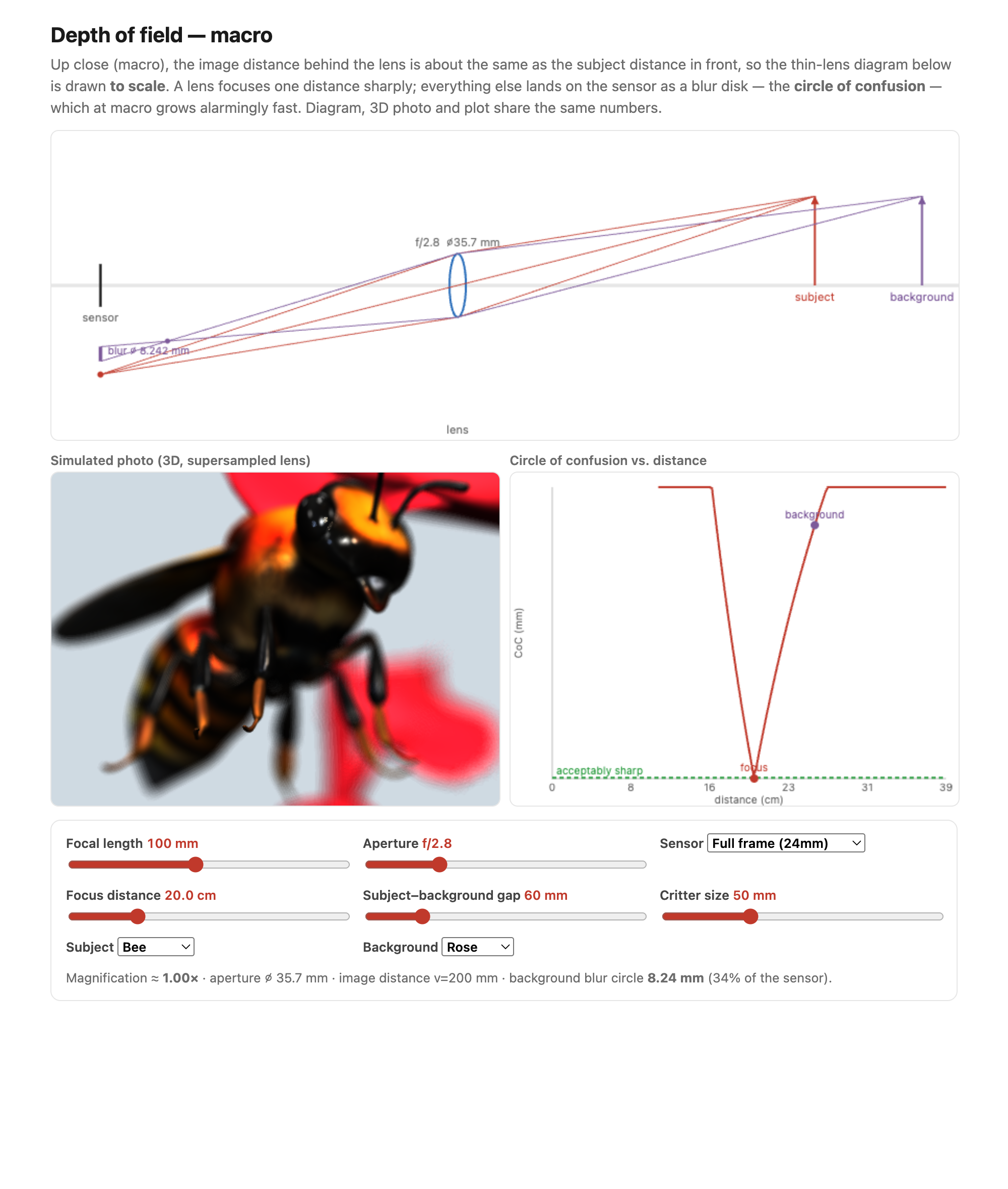
• **aperture — changes the picture**: range $\sim f/1.4$ to $f/22 \approx$ **2.5 orders** ($k\propto 1/N_f^2$). **Con:** it changes **depth of field** — the bracket frames would have *different focus blur*, breaking the "only the exposure changes" assumption. Use only when desperate.

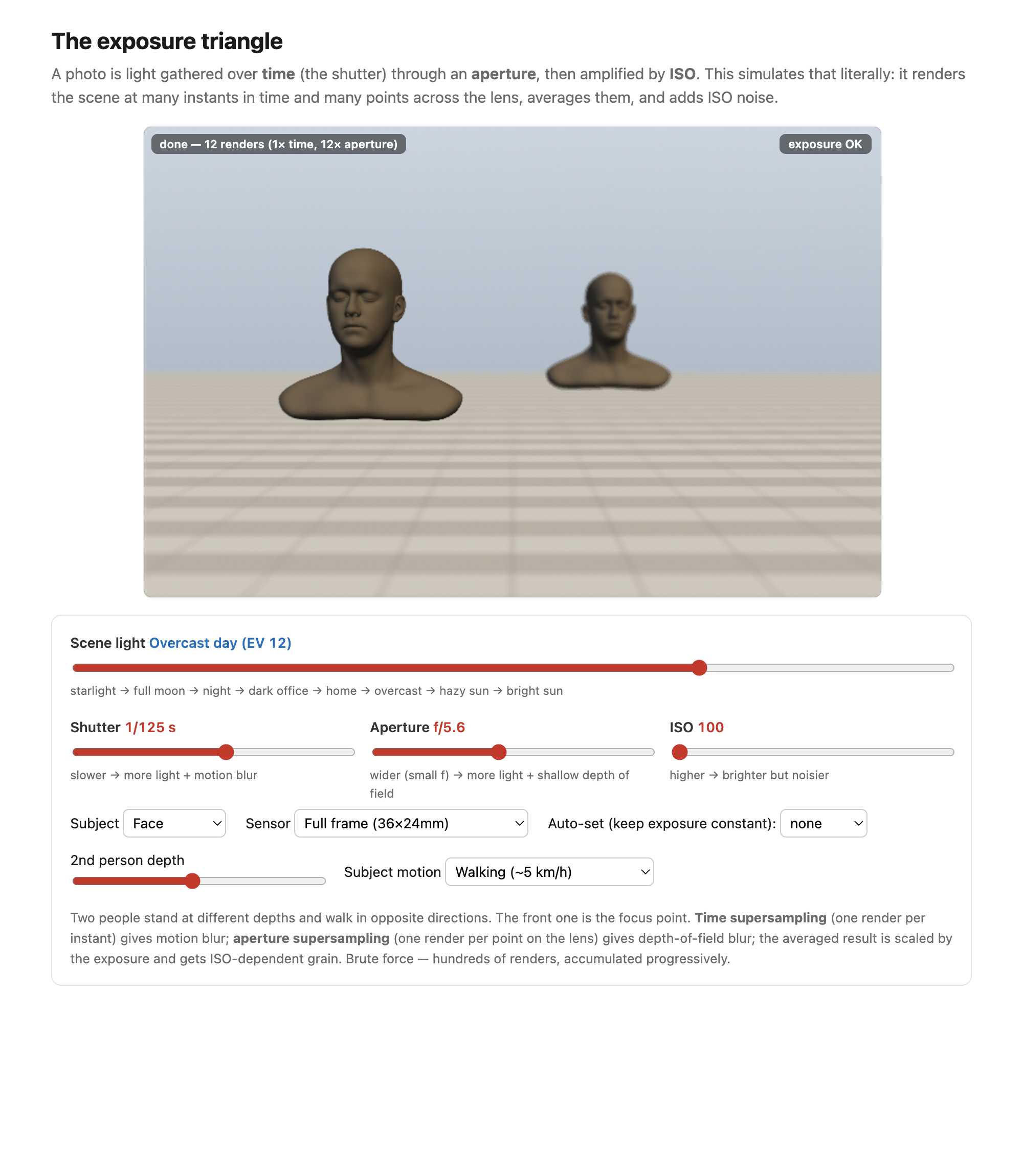
• **ISO — amplifies, doesn't collect**: range $\sim$100 to 1600 ≈ **1.5 orders**. ISO is **analog/digital gain applied after capture**, not more light — so it scales signal *and* read-noise-referred terms and generally **raises noise**. Useful when desperate, but a poor way to extend range on its own. (Hasinoff's insight, below, is that ISO *is* a useful degree of freedom once you model noise properly.)

• **neutral-density (ND) filter — darkens the world**: up to $\sim$4 densities ≈ 4 orders, **stackable**. **Cons:** not perfectly neutral (introduces a **color shift**), imprecise, and you must **touch the camera** to add it (risking shake → needs re-registration). **Pro:** works with strobe/flash where shutter can't, a good complement when desperate.

• **the takeaway** (ties to **L7** — stops): exposure is **counted in stops** (factors of 2, additive in log space), and the clean way to walk the radiance axis is **shutter**; the other knobs trade a side effect (DoF, noise, color) for range and are fallbacks. *Forward-ref:* which exposures to pick — not just *how* to vary, but the **optimal set** — is the *Optimizing the capture and merge* section (Hasinoff).

• **the merge assumes static + registered**: the basic merge assumes **only the exposure changes — no motion**. Hand-held bracketing breaks this; align first (Ward 2003's **median-threshold bitmap**, MTB — a contrast-robust alignment that compares images thresholded at their median, accelerated on a pyramid) and reject **ghosts** from moving objects. Cross-ref [[#Image alignment]]; the burst-imaging chapter makes robust alignment central.

• **on-chip HDR — the sensor does the merge (no software bracket)**: everything above assumes *software* fuses a bracket of separate frames. But **on-chip HDR is now an industry-wide sensor capability** — many modern image sensors **produce a high-dynamic-range signal directly, on-chip**, folding the "capture several slices and combine" step into the readout itself. **Sony** is a prominent example (its DOL / dual-read schemes, below), but **OmniVision**, **Samsung (ISOCELL)**, and **onsemi** and other automotive vendors (split-pixel designs) all do on-chip HDR by various strategies — it's a hardware strategy, not one vendor's feature. This is the hardware cousin of bracketing: instead of $N$ frames merged in post, the slices are captured and combined *inside the sensor / ISP*, so the photographer gets one wide-DR raw out. The main strategies differ in **how** they multiplex the dynamic range — in **time**, in **space**, or in **gain**: [`fig-hdr-sensor-strategies`]

• **DOL-HDR / "double read" (digital overlap)** — read the same exposure twice, or interleave **long + short** exposures line-by-line, then combine; the long read recovers shadows, the short read the highlights. This is the Sony **"double read."** *Time-multiplexed:* the long and short captures are not simultaneous, so anything moving between them **ghosts** (motion artifacts) — the same de-ghosting problem as a hand-held bracket, now inside one frame.

• **dual-conversion-gain (DCG)** — each pixel can be read at **two readout (conversion) gains**: high gain for a low noise floor in the shadows, low gain for more full-well headroom in the highlights; the two reads are merged. *Gain-multiplexed:* both reads see the **same instant**, so it is the **cleanest** option — no motion artifacts, no resolution loss — but the extra range it buys is **bounded** by the gain spread.

• **split-pixel / dual-photodiode** — each photosite carries a **large + small** sub-photodiode: the large one saturates early (shadows/midtones), the small one keeps reading into bright highlights. Common in **automotive** sensors (sun-glare, tunnel exits). *Space-multiplexed:* costs **resolution / fill-factor and SNR** (the small diode is noisy), but both sub-pixels are exposed simultaneously, so no motion ghosting.

• **lateral-overflow / LOFIC / voltage-domain tricks** — add **extra charge capacity** per pixel (a lateral-overflow integration capacitor that catches the charge spilling past the photodiode's well), extending full-well in the **voltage/charge domain** without a second exposure.

• **spatially-varying exposure (SVE / "assorted pixels")** — bake **different sensitivities into neighbouring pixels** (an exposure mosaic, like a Bayer pattern but for ND), then demosaic into an HDR image — **Nayar & Mitsunaga**. *Space-multiplexed:* trades **resolution** for range, single-shot so no motion artifacts.

• **logarithmic / companding sensors** — a pixel whose response is **log (or piecewise-companded)** in radiance, capturing many decades in one read at the cost of **lower contrast resolution / fixed-pattern non-uniformity** in any given band.

• **the trade-off, in one line**: **time-multiplexed** schemes (DOL double-read) buy range with **motion artifacts**; **space-multiplexed** schemes (split-pixel, SVE/assorted pixels) buy it with **resolution / SNR**; **gain-domain** (DCG) is the **cleanest** — same instant, full resolution — but its extra range is **bounded**. The software **HDR+ burst** of the next chapter ([[#Application to cell phones: HDR+ and burst imaging]]) sits at the opposite end: maximal flexibility and denoising-for-free, paid for in compute and alignment. This is the **computational-sensor** trade space — push the work into silicon or into software — developed in [[Advanced computational photography]] (cross-ref). [`fig-hdr-sensor-strategies`]

• **the calibration question**: to merge, you must know how a pixel value $z_i$ relates to scene radiance — i.e. recover the **exposure factors** $k_i$ (or their ratios) and, if the capture is non-linear, the **camera response curve** $f$ where $z = f(k\,L)$. Two regimes: **linear capture** (easy, a ratio) and **non-linear capture** (regression on pixels seen at multiple exposures).

• **linear case — just a ratio**: if the images are **linearly encoded** (raw, or un-gamma'd — `dcraw -g 2.2 0` gives linear-ish; **L2**: do radiometry in linear light), then in any non-clipped, non-noisy pixel $I_i = k_i L$. So for a pair of adjacent exposures the radiance cancels: $I_i/I_j = k_i/k_j$ — *the same value at every good pixel* if linearity holds. Estimate it robustly: $k_i/k_j=\mathrm{median}_{x:\,w_i,w_j>0}\big(I_i(x,y)/I_j(x,y)\big)$, taking the **median** over pixels where **both** images are reliable. **Chain** the pairwise ratios to get every $k_i/k_0$ — you only ever recover exposure up to **one global scale factor** (which is fine: radiance maps are relative unless you photometrically calibrate). [`fig-pixel-ratio-calibration`]

• *practical note:* you can also just read $k_i$ from the **EXIF exposure data** ($t_i$, $f$, ISO); the ratio-from-pixels method is the fallback when the metadata is missing or the response is suspect, and it's more robust because it's measured from the actual data.

• **non-linear case — recover the response curve (Debevec–Malik 1997)**: real cameras (and film, and JPEG) apply a **non-linear response** $f$ (gamma, tone curve, film characteristic). Then $z_i = f(k_i L)$ and you must recover $f$ (equivalently its log-inverse $g=\ln f^{-1}$) before you can merge. The trick: a pixel imaged at **several exposures** gives several $(z_i, t_i)$ pairs constraining the *same* radiance — that over-determination pins down the curve. Write, in the log domain, $g(z_i) = \ln L + \ln t_i$. The unknowns are the curve $g(\cdot)$ (one value per possible pixel level, e.g. 256) and one $\ln L$ per pixel. Solve a **linear least squares** over all pixels and exposures, with two riders: a **smoothness penalty** on $g''$ (a real response is smooth), and a **reliability weight** $w(z)$ down-weighting near-clip and near-noise samples. Recovered only up to **one additive constant** (= the global scale). [`fig-response-curve-debevec`]

• **Mitsunaga–Nayar 1999 — even less is assumed**: models the response as a **low-order polynomial** and recovers it (and the unknown exposure ratios jointly) by **radiometric self-calibration** — you don't even need to trust the EXIF exposure ratios. Same spirit: pixels seen at multiple exposures over-determine the curve; fit a smooth response. (Mann & Picard 1995's "comparametric" / Wyckoff work is the earlier multiple-exposure precursor.)

• **why regression beats raw ratios** (the cleaner-way bridge): a **robust regression** for $g$ and $L$ avoids brittle per-pair ratios, **directly models uncertainty due to noise** (heavier weight where SNR is high), and **generalizes to the full non-linear response** in one framework. This is the seam into *Optimizing the merge*: once you've written it as least squares, the *right* weights are inverse-variance — the next two sections.

• **encoding note (L2)**: merging is an **additive** operation in radiance, so it must be done in **linear light** (or, equivalently, the log-radiance domain of Debevec). Gamma/tone-curved values are *not* proportional to radiance and would merge wrong — un-apply the response first. (The *display* side, by contrast, lives in a perceptual/log space — that's tone mapping, elsewhere.)

• **the assembly recipe** (three steps): (1) figure out the **scale factor** $k_i$ between images — from EXIF or pixel ratios (previous section); (2) compute a **weight map** $w_i(x,y)$ for each image marking which pixels are usable; (3) **reconstruct** the radiance per pixel as a **weighted combination** of the rescaled observations. [`fig-weight-triangle`]

• **which pixels are useful — the reliability mask**: at each pixel, an exposure's value is trustworthy only if it is **neither clipped nor noise-dominated**. Reject **clipped** highlights (e.g. $z > 0.99$) — they only tell you "at least this bright," not how bright. Reject **too-dark / too-noisy** shadows (e.g. $z < 0.002$) — the read-noise floor swamps the signal. What's left is the usable band. (P-set 5 uses **binary** $w\in\{0,1\}$, extensible to a smooth scalar; weights can differ per color channel.)

• **the merge — a weighted average in radiance**: rescale each usable observation to radiance by dividing out its exposure factor, $z_i/t_i$ (or $z_i/k_i$), then average, weighted by reliability:

$$\hat L(x,y)=\frac{\sum_i w(z_i)\,z_i/t_i}{\sum_i w(z_i)}.$$

In the non-linear (Debevec) case, the identical average runs in the **log domain** on the recovered curve: $\ln\hat L=\big(\sum_i w(z_i)\,(g(z_i)-\ln t_i)\big)\big/\big(\sum_i w(z_i)\big)$. Either way it is a **reliability-weighted mean** — and where several exposures overlap, the averaging also **denoises** (the $1/\sqrt N$ effect of [[#Denoising by averaging]], reliability-weighted). [`fig-weight-triangle`]

• *pseudocode*: the merge as one per-pixel pass over the bracket — divide out each exposure factor, accumulate by reliability weight, normalize, with the all-bad fallback to the brightest/shortest frame.

• **edge case — pixels bad in *every* exposure**: a pixel may be **clipped in all** images (a light source) or **noise-dominated in all** (deepest shadow). Don't discard it: **keep clipped pixels in the *brightest*-exposed image** (the one shot long enough to have *some* value there — for the darkest part) and **keep dark pixels in the *shortest* exposure**. Careful with the threshold implementation: the literal values $0.0$ / $1.0$ must actually be *kept* for these fallback images, not rejected. (Mind the direction: dark pixels of the *brightest* image, bright pixels of the *darkest* — not the reverse.)

• **the connection to denoising and to fusion** (the unifying view): the unweighted, single-radiance-band case of this average is exactly **average-to-denoise** ([[#Denoising by averaging]]) — HDR merge generalizes it with per-observation reliability/SNR weights. A *different* philosophy is **exposure fusion** (Mertens, Kautz & Van Reeth 2007): skip the radiance map entirely — score each bracket pixel by a **per-pixel quality** (well-exposedness, local contrast, saturation), then **blend the bracket directly in a Laplacian pyramid** weighted by those scores. No response-curve recovery, no HDR float map, no separate tone-mapping step — the multi-scale (pyramid) blend hides the exposure seams and yields a *displayable* image in one shot. Cross-ref the pyramid-blend machinery in [[Linear pyramids and wavelets]]; fusion is the pragmatic "merge straight to a viewable image" alternative to "build an HDR map, then tone-map."

• **the better question** (beyond binary weights): when **multiple exposures both see a pixel validly**, they have **different noise**. Plain binary masks throw away information — using *only* the least-noisy observation gets no $1/\sqrt N$ benefit; there must be a way to use the noisier one *at least a little*. The principled answer: weight by **reliability = inverse noise variance**.

• **the two-observation derivation** (the kernel of it): given two unbiased estimates $x,y$ of the same quantity with variances $\sigma_x^2,\sigma_y^2$, combine as $\hat L = a x + (1-a) y$. Its variance is $a^2\sigma_x^2 + (1-a)^2\sigma_y^2$; differentiate w.r.t. $a$, set to zero → $a^\* = \dfrac{\sigma_y^2}{\sigma_x^2+\sigma_y^2}$. The **optimal combination weights each estimate by the inverse of its variance** (check: equal variances → $a=1/2$, the plain average; one estimate far noisier → it gets little weight but not zero). Generalize: $w_i = 1/\sigma_i^2$, giving $\hat L = \dfrac{\sum_i (z_i/k_i)/\sigma_i^2}{\sum_i 1/\sigma_i^2}$ — **inverse-variance (minimum-variance) weighting**, the BLUE estimator. [`fig-naive-vs-optimal-weights`]

• **plug in the camera's noise model**: variance is dominated by two terms (FUNDAMENTALS — Noise): **photon (shot) noise** with variance $\propto$ signal (dominates in the highlights) and **read noise** with constant variance (dominates in the shadows): $\sigma^2(x) = a\,x + \sigma_{\text{read}}^2$, where $a$ and $\sigma_{\text{read}}$ depend on camera and ISO. Calibrate by shooting repeated frames (variance across the stack) or derive it on paper. Now the merge weights aren't a hand-drawn hat — they come from physics.

• **what falls out** (a clean, slightly surprising result): rescaling an observation by $1/k_i$ to radiance amplifies **both signal and noise**, so $\mathrm{Var}(z_i/k_i)\approx \sigma_i^2/k_i^2$. Working the algebra through the inverse-variance formula for the **photon-noise-only** case: the per-pixel radiance $L$ and the slope $a$ are common to every term (they appear in numerator and normalizer) and **cancel**, and the two $k_i$ factors cancel too — so **all pixels of a given exposure get the same weight**, $w'_i \propto k_i$ (longer/brighter exposures, with relatively less photon noise, weighted up). The images aren't literally rescaled to radiance in the sum, but the normalization makes it equivalent. (With **read noise** included the cancellation is incomplete and the optimal weights *do* vary per pixel — read noise is what makes the optimum genuinely spatially varying.) Still reject clipped/dark pixels with the binary mask, *then* weight the survivors by inverse variance. [`fig-naive-vs-optimal-weights`]

• **Hasinoff–Durand–Freeman 2010 — optimizing the *capture set*, not just the merge**: don't stop at optimal *weights* for a *given* bracket — choose the **optimal set of exposures** to shoot. With a full noise model (photon + read, and **exploiting ISO** as a real degree of freedom), pick the shutter/ISO sequence that **maximizes worst-case SNR** across the scene's brightness range under a fixed time budget. The counter-intuitive result: the SNR-optimal set often uses **higher ISO and shorter exposures** than naive bracketing — e.g. for one scene, standard bracketing ISO 100 (1/100, 1/25, 1/6 s) is beaten by an SNR-optimal ISO 3200 (1/3200, 1/125, 1/5 s), gaining $\sim$12 dB in the dark regions and approaching the **ideal HDR sensor** curve. [`fig-hasinoff-snr-optimal-set`]

• **the through-line into cell phones**: Hasinoff's "fewer/shorter/higher-ISO, then merge optimally" logic — *underexpose to avoid clipping and to freeze motion, recover the rest by computation* — is exactly the philosophy of **HDR+** (next section), where the bracket becomes a **burst of identical underexposed raws** merged for denoising *and* range at once. (Other refs in this vein: Granados et al. 2010, optimal per-pixel weights from the full noise model; Ward 2003, robust capture with registration + ghost/flare removal.)

• **the phone's predicament**: a tiny sensor (small photosites → low full-well capacity → low single-shot DR and high relative noise — **L15**), **no tripod**, an unsteady hand, and a scene with people moving. Classic bracketing — a few *different* exposures, assume static — fails: the long exposure blurs from hand shake, subjects move between frames (ghosts), and the small sensor's shadows are noisy anyway. [`fig-burst-vs-bracket`]

• **the HDR+ move (Hasinoff 2016)**: replace the bracket with a **burst of many *identical* frames**, each at the **same short, deliberately under-exposed** raw exposure. Short exposures **freeze motion** (no per-frame blur) and are easy to align; *many* of them, **averaged**, beat the noise down by $1/\sqrt N$ — recovering the shadow detail you'd otherwise have gotten from a long exposure, but without the blur. The burst does double duty: **denoising** (the $1/\sqrt N$ of [[#Denoising by averaging]]) **and HDR** (range recovered from the merge) in **one** operation. This is **L14** on a phone — capture the full set (the burst), decide later (merge + tone-map). [`fig-burst-vs-bracket`]

• **why *under*expose — the irreversibility asymmetry** (the crux): the two failure walls are **not** symmetric. A **clipped highlight is gone forever** — once a photosite saturates, the information is destroyed and no merge recovers it. A **dark-but-unclipped shadow is only noisy**, and noise is **recoverable** by averaging $N$ frames. So bias the exposure **down**: pick $k$ small enough that even the **brightest** scene radiance stays below clipping ($k\,L_{\max}<1$), guaranteeing **highlight headroom**, and pay for it with extra shadow noise that the burst merge then removes. You trade a *recoverable* problem (noise) for avoiding an *unrecoverable* one (clipping). [`fig-why-underexpose`]

• **this is Hasinoff 2010 on a phone**: it's exactly the **SNR-optimal capture set** logic — shorter exposures, higher effective ISO, recover by computation — instantiated as "one short exposure repeated $N$ times." The 2010 paper said *how to choose the optimal set*; HDR+ says *for a phone, the optimal set is a uniform under-exposed burst*, because that also solves motion and alignment.

• **the pipeline** (end to end): **capture** a burst of $N$ under-exposed raw frames (raw = linear, pre-demosaic, **L2**) → **select a reference** (a sharp, well-exposed-enough frame, often an early one) → **align** every other frame to the reference (tile-based, sub-pixel) → **robustly merge** the aligned frames **in the raw domain** → emit **one denoised, high-DR raw** → **demosaic**, then **tone-map** and finish (the displayable JPEG). The key architectural choice: **merge happens in raw, before demosaicking**, so denoise + HDR are a single operation on the cleanest (linear, mosaiced) data. [`fig-hdrplus-pipeline`]

• **the merge is a robust weighted average** — the [[#HDR merging]] merge with one addition: $\hat L = \sum_i w_i\,I_i(W_i^{-1}x)/\sum_i w_i$, where $W_i$ is the estimated alignment of frame $i$ and the weight $w_i$ combines **inverse-variance reliability** (from the noise model) with **outlier rejection** — a frame (or tile) that *disagrees* with the reference (because a subject moved, or alignment failed) is **down-weighted or dropped**, so it can't contribute a ghost. Conceptually a per-frequency **Wiener-style merge** in the tile transform: where frames agree, average hard (full denoise); where they disagree, trust the reference (no ghost). [`fig-ghost-from-misalignment`]

• **alignment is the whole game** (and ghosts are its failures): mis-registration turns the helpful average into **blur and double-images**. HDR+ aligns in **tiles** (a coarse-to-fine, pyramid search per tile) to handle locally-varying motion, and the **robust** merge is the safety net for the residual motion the alignment can't undo (occlusion, fast subjects). The trade is explicit: more aggressive averaging = more denoising but more ghost risk; the robustness weight tunes it per pixel. (Cross-ref [[#Image alignment]]; this is the same MTB/pyramid-search lineage as Ward 2003, made local and sub-pixel.)

• **why raw, before demosaic**: doing the merge on **linear raw** keeps the noise model simple and correct (photon + read, **L15**), lets the merge *also* serve as the demosaic's denoiser, and avoids baking in the non-linear tone curve before the additive average (**L2** — average in linear light). Tone mapping comes **after** the merge (local tone mapping; HDRnet / Gharbi 2017 learns this step on a **bilateral grid** — forward-ref to [[Edge-preserving techniques]] and [[Deep learning]]).

• **the same substrate, one knob turned**: HDR+ aligns and merges a burst to gain **SNR and range**. **Burst super-resolution** (Wronski et al. 2019, the Pixel "Super Res Zoom") aligns and merges the *same kind of burst* to gain **resolution**. The only difference that matters is **sub-pixel** alignment: the unavoidable **hand tremor** between frames shifts the scene by fractions of a pixel, so each frame samples the continuous scene on a slightly **offset grid** — fuse them on a **finer grid** and you recover detail beyond a single frame's sampling. [`fig-burst-superres-link`]

• **aliasing becomes the signal**: a single frame's sampling **folds** high frequencies (aliasing — normally a defect); the sub-pixel-shifted frames let you *separate* those folded frequencies, turning aliasing into recovered resolution. This is **reconstruction-based** super-resolution (genuine measured detail), not hallucination — cross-ref the reconstruction-vs-hallucination axis in [[Single-image computational photography#Reconstruction vs hallucination]]. It even **replaces demosaicking**: the color mosaic's own per-channel offsets, combined across the burst, reconstruct full color directly. [`fig-burst-superres-link`]

• **the unifying statement** (close the chapter): HDR merge, burst denoising, and burst super-resolution are **one operation** — *align a burst, then robustly merge* — with the dial set to recover **range** (HDR+), **SNR** ($1/\sqrt N$ denoise), or **resolution** (sub-pixel super-res), and usually **all three at once** on a modern phone. The full super-resolution treatment (the prior, the ill-posedness, the fusion math) lives in [[Single-image computational photography]]; here it closes the multiple-exposure arc — *capture the set, align, merge, decide later* (**L14**), beating the single-shot limits of **L15** by computation.

• **the setup**: you stand in one place and **pan the camera** across a scene, taking overlapping frames. Choose one frame as the **reference**; reproject (warp) the others into its coordinate system; blend the overlaps. The output is a virtual **wide-angle** view. [`fig-pano-4clicks`]

• **the one rule** — pure **rotation about the optical centre**. The camera may rotate freely (pan, tilt, roll) but its **viewpoint must not move**. If you keep the optical centre fixed, every pair of views is related by a single homography (derived below) *regardless of scene geometry*. [`fig-pano-rotate-vs-translate`]

• **why translation breaks it**: if you *walk* (translate the optical centre), near and far objects shift by **different** amounts — **parallax**. There is then no single 2D map between the views; you'd need the depth of every pixel (i.e. actual 3D reconstruction). The slogan for the reader: **"rotate, don't walk."** The one exception is a **planar scene** (next-to-last section) — there a homography works *even if you translate*, because a plane has, in effect, one depth law.

• **forward-pointer**: the *warping itself* — forward vs inverse warp, resampling, antialiasing — and the closely-related **perspective-distortion correction** are developed in [[Slopendium/09 Motion, warping, and video|Motion, warping, and video]]. Here we only need the **geometry** (which $H$) and how to **solve** for it.

• **the pinhole model**: a 3D point $(x,y,z)$ in the camera frame images to $(x/z,\,y/z)$ on the plane $z=1$. **Projection is division by depth.** Far things look small because you divide by a bigger $z$. [`fig-pinhole-divide-by-z`]

• **rotating the camera = rotating the world the other way**: to project a point into a camera that has been rotated by $R$, apply $R^{-1}$ (equivalently $R$ to the ray) then divide. So a rotated view of the *same* scene is: rotate the 3D points, then re-project (divide by the new $z'$).

• **the trap we're about to escape**: this recipe needs the 3D point — and for stitching we only have the **first image's pixels**, not their depths $z$. Are we stuck? (No — that's the next section.)

• **the key observation** — *all points along one viewing ray reproject to the same place.* A pixel $(x,y)$ in image 1 is the image of an entire **ray** of 3D points $(tx,ty,t)$ for every depth $t$. Rotate that whole ray by $R$ and re-project: the **divide by $z'$ removes the common factor $t$**. Every point on the ray lands on the *same* pixel in the rotated view. So the destination pixel **does not depend on depth at all**. [`fig-depth-cancels-ray`]

• **therefore pick $z=1$**: since depth doesn't matter, treat each pixel as the point $(x,y,1)$ — pretend the image is a plane at distance 1 — rotate by $R$, divide by the new third coordinate. That is the entire mapping. We *chose* a depth only for convenience; any choice gives the same answer. [`fig-homog-coords-1d` shows the 1D toy: reprojecting points to another line is linear and depth-free]

• **the equation** — chaining "un-project (apply $K^{-1}$), rotate ($R$), re-project (apply $K$)" gives the view-to-view map

$$\mathbf{x}' \simeq H\,\mathbf{x}, \qquad H = K\,R\,K^{-1},$$

where $K$ is the camera's intrinsics (focal length, principal point) and $\simeq$ means "up to scale" (you still divide by the last coordinate). **Crucially, no $z$ appears in $H$** — depth has cancelled. For normalised coordinates ($K=I$) it's just $H=R$ acting on rays $(x,y,1)$.

• **the punchline to state plainly**: *for a camera rotating about its optical centre, the relationship between two images is a homography that is independent of the scene.* No depth, no 3D model, no parallax — one $3\times3$ matrix relates the views everywhere. This is the chapter's central idea and the reason panorama stitching is a clean linear problem. (Reused in [[#Automatic panorama stitching from multiple views and feature matching|automatic stitching]] and in perspective correction.)

• **homogeneous coordinates** — represent a 2D point $(u,v)$ by **three** numbers $(x,y,w)$ with $u=x/w,\ v=y/w$. Recover the Euclidean point by **dividing by the last coordinate**. All scalings $(wx,wy,w)$ name the same point → coordinates are defined **up to scale**. Motivations: they make **perspective** (the divide) and **translation** expressible as a single matrix multiply, and they're exactly "treat the image as a plane at $z=1$ in 3D." [`fig-homog-coords-1d`]

• **a homography** is any $3\times3$ matrix $H$ acting on homogeneous coordinates: compute $\mathbf{x}'=H\mathbf{x}$ (plain matrix multiply), then **divide by $w'$** to read off image coordinates. It is the most general **projective mapping of a plane** — and, per the previous section, exactly the camera-rotation map. [`fig-homography-quad`]

• **what it does geometrically**: maps the input **rectangle to an arbitrary quadrilateral**; parallel lines need not stay parallel (they can converge to a vanishing point), but **straight lines stay straight**. Same as "project the plane, rotate, re-project." [`fig-homography-quad`]

• **8 degrees of freedom**: $H$ has 9 entries but is defined **up to scale** ($H$ and $kH$ give the same map, since $(kw'x',\dots)$ and $(w'x',\dots)$ are the same Euclidean point) → **8 DOF**. This is why **4 point correspondences** (8 numbers) are exactly enough to pin it down.

• **the per-point formula** (writing $H=\begin{psmallmatrix}a&b&c\\ d&e&f\\ g&h&i\end{psmallmatrix}$): $\ x'=\dfrac{ax+by+c}{gx+hy+i},\quad y'=\dfrac{dx+ey+f}{gx+hy+i}.$ The denominator $w'=gx+hy+i$ is the perspective divide; $g,h$ are what make lines converge (zero $g,h$ → an affine map, no perspective).

• **the goal**: given $\ge4$ matched point pairs $\mathbf{x}_i\leftrightarrow\mathbf{x}_i'$, find $H$ mapping each $\mathbf{x}_i$ to $\mathbf{x}_i'$. In manual stitching the user supplies these by clicking; automatically they come from feature matching (next chapter).

• **make it linear**: the relation $\mathbf{x}'\simeq H\mathbf{x}$ looks nonlinear because of the divide, but **cross-multiplying** by the denominator clears it. Each correspondence yields **two linear equations** in the 9 unknown entries of $H$ — e.g. one of them is $a x + b y + c - x'(g x + h y + i)=0$. Stack them: $A\mathbf{h}=\mathbf{0}$, where $\mathbf{h}$ is the 9-vector of $H$'s entries. With 4 pairs you get $8$ equations.

• **the scale freedom** (and how to kill it): $\mathbf{h}=\mathbf{0}$ is a trivial solution and $H$ is only defined up to scale, so you must **fix the scale**:

• **dirty version** — assume $i\neq0$ and **set $i=1$** (true unless the camera is rotated ~90°). Then 8 unknowns, $A\mathbf{x}=\mathbf{b}$ with a nonzero right side; solve directly (4 pairs) or by **least squares** if you have more pairs (overconstrained $\arg\min\lVert A\mathbf{x}-\mathbf{b}\rVert^2$, the normal equations $A^\top A\mathbf{x}=A^\top\mathbf{b}$). Good enough for a problem set.

• **clean version** — keep all 9 unknowns and solve the homogeneous $A\mathbf{h}=\mathbf{0}$ by **SVD**: $H$ is the **singular vector with the smallest singular value** (the null space). No arbitrary assumption about $i$. [link to [[Linear Inverse Problems and Regression]] for the SVD null-space solve]

• **overdetermined is good**: more than 4 correspondences → solve in **least squares**; this averages out clicking noise. (And, in the next chapter, lets **RANSAC** discard wrong matches before the final fit.)

• **a fitting analogy**: just like fitting a line $x'=ap+b$ from many noisy $(p,x')$ pairs, different correspondence sets can yield the *same* $H$; the unknowns are $H$'s coefficients, the data are the point pairs.

• **pick a reference, warp the rest**: choose one image's coordinate frame as the canvas; for every other image, warp it into that frame using its homography (warp one-by-one toward the reference). The union is the wide panorama; pixels no part of any image reaches stay **black**. [`fig-pano-warp-to-reference`]

• **inverse warp** (the right way to resample): loop over **output** pixels $(x,y)$, map *back* into the source with $H^{-1}$, then divide and sample (with interpolation/antialiasing) — this guarantees every output pixel is filled, no holes. (Forward warp leaves gaps.) The full forward-vs-inverse warp and resampling story is in [[Slopendium/09 Motion, warping, and video|Warping]].

• **bounding box**: to size the canvas, **forward**-map the source corners through $H$ to see where the warped image lands; then **inverse**-warp to fill the output. (Forward for the bbox, inverse for the pixels.)

• **then blend** — the warped images overlap and won't match exactly (exposure, vignetting, tiny misalignment); merging them seamlessly is the [[#Blending|Blending]] section's job (feathered/two-scale/Poisson). Here we just place them.

• **other projections** (pointer): warping everything onto one flat reference plane stretches badly for very wide fields of view; **cylindrical / spherical** projections (and "little planet" stereographic) are the fix — covered later under *Other projections*.

• **the planar twin**: everything above needed *pure rotation* because general scenes have depth. But if the scene is a **single plane**, a homography relates **any** two views of it — *even when the camera translates* — because a plane imposes one depth relationship across the whole surface (no independent per-pixel depth). A plane photographed from any viewpoint maps to a plane by a homography.

• **document flattening (rectification)**: photograph a page, whiteboard, painting, or building façade at an angle and it appears as a **keystoned quadrilateral**. Click (or detect) its **four corners**, set them as correspondences to a target rectangle, solve for $H$, and **warp** → a fronto-parallel, "scanned" version with verticals vertical and the page rectangular. [`fig-doc-flatten`]

• **document merging**: to capture a large document (or a whiteboard too big for one frame), shoot **overlapping** planar patches and stitch them with planar homographies — the same pipeline as a panorama, but the homography is justified by the **planar scene** rather than by pure rotation. Useful for book scanning, mosaicing microscope slides, aerial/satellite image tiles of (locally) flat ground.

• **same machinery, different justification** — worth stating for the reader: panoramas (rotation) and document rectification/merging (plane) are *the same homography solve*; only the geometric reason the homography is valid differs. (Perspective-distortion correction — making a building's verticals parallel — is the same trick and is developed in [[Slopendium/09 Motion, warping, and video|Warping]].)

• **the dead end** (worth showing): the old way matched images **densely** — try all translations, compute the sum-of-squared-differences (SSD) over all pixels, keep the best. For a **homography** that means discretising **8 coefficients** — combinatorially hopeless — and each trial requires a full warp + SSD. Even reduced to a couple of rotational DOF it's restrictive, slow, and **not robust** to moving objects or distortion. [`fig-feature-pipeline` motivates the alternative]

• **the modern idea — sparse matching**: ignore uniform regions; focus on a few **very distinctive points** (interest points), match them **locally** (which point ↔ which point), and add machinery to be **robust to local mistakes**. Sparse, fast, robust.

• **the two problems to solve** (state them as the chapter's skeleton): **(1) repeatable detection** — detect the *same* scene point **independently** in each image (if a point is found in one image but not the other, it can never match); **(2) distinctive description** — for a detected point, **recognise** its correspondent in the other image, via a descriptor that's similar for the same scene point and different for others. [`fig-corner-flat-edge`]

• **the discipline to emphasise**: detection and description run **independently in each image**. Only **at the very end**, given a bag of (point, descriptor) features per image, do we compute correspondences. We analyse the detector/descriptor on *corresponding* scene points only to *check* they'd behave consistently.

• **what makes a good keypoint**: a point you can **localise precisely** and **re-find reliably**. The test (Moravec's idea): slide a small window a little in **any** direction and measure how much the patch changes. **Flat** region → no change in any direction (not localisable); **edge** → no change *along* the edge (slides freely → ambiguous); **corner** → **large change in every direction** → uniquely pinned down. *Corners make the best keypoints.* [`fig-corner-flat-edge`]

• **quantify it**: the windowed change under a shift $(u,v)$ is $E(u,v)=\sum_{x,y} w(x,y)\,[I(x+u,y+v)-I(x,y)]^2$, with $w$ a box or Gaussian window. Computing this for all shifts is costly — so **Taylor-expand** $I(x+u,y+v)\approx I+I_xu+I_yv$ to get a **quadratic form**: $E(u,v)\approx \begin{psmallmatrix}u&v\end{psmallmatrix}M\begin{psmallmatrix}u\\ v\end{psmallmatrix}$.

• **the structure tensor** $M=\sum_{x,y} w\begin{psmallmatrix}I_x^2 & I_xI_y\\ I_xI_y & I_y^2\end{psmallmatrix}$ (a.k.a. second-moment matrix) packs the local gradient statistics into a $2\times2$ symmetric matrix. Its **eigenvalues** $\lambda_1,\lambda_2$ are the change rates along the two principal directions; the iso-$E$ contour is an **ellipse** with axes $\propto\lambda^{-1/2}$. [`fig-harris-eigen-ellipse`]

• **classify by eigenvalues**: both small → **flat**; one large, one small → **edge** (the freely-sliding direction has tiny $\lambda$); **both large** → **corner**. [`fig-harris-eigen-ellipse`]

• **the Harris response** (avoid computing eigenvalues explicitly): $R=\det M - k(\operatorname{tr}M)^2 = \lambda_1\lambda_2 - k(\lambda_1+\lambda_2)^2$, $k\approx0.04$–$0.06$. $R$ is large-positive at corners, large-negative on edges, small in flat regions. (**Shi–Tomasi** variant: just use $R=\min(\lambda_1,\lambda_2)$.)

• **the algorithm**: compute gradients $I_x,I_y$; form $M$ per pixel (windowed sums of products); compute $R$; **threshold** $R$; keep **local maxima** of $R$ (non-max suppression over a $k\times k$ neighbourhood) → the detected corners. [workflow figure within `fig-harris-eigen-ellipse` family]

• **invariances** (what survives between two views): **rotation** — the ellipse rotates but its **eigenvalues don't change**, so $R$ is rotation-invariant (a clean example of eigen-analysis giving a rotation-invariant quantity); **intensity** — uses only **derivatives**, so invariant to a brightness shift $I\to I+b$, and partially to scaling $I\to aI$ (the threshold is the catch). **Not invariant to scale**: zoom in and a corner's neighbourhood looks like an edge → it gets classified differently. That failure motivates SIFT. [`fig-harris-not-scale-invariant`]

• **the simple descriptor** (the basic, pre-SIFT version — enough for a first system): take the **$k\times k$ patch** of luminance around the corner; **blur** slightly (reduce sampling/aliasing); **subtract the mean and divide by the standard deviation** (kill brightness/contrast differences from exposure, vignetting, clouds). The descriptor is just those $k\times k$ normalised numbers.

• **brute-force matching**: for each feature in image 1, scan all features in image 2 and keep the one with smallest descriptor **SSD** $d=\lVert\mathbf{f}_i-\mathbf{f}_j\rVert^2$. This gives every corner a match — *including many wrong ones* (even points in non-overlapping regions get a "match"). Two cleanups follow: the **ratio test** (next-but-one) and **RANSAC**.

• **the goal**: a detector that finds the same point across **scale and rotation** changes, and a descriptor that's correspondingly **invariant** — so wide-baseline, zoomed, rotated views still match. SIFT (Lowe 2004) is the canonical answer. [`fig-feature-pipeline`]

• **scale selection via scale-space**: blur the image with Gaussians of increasing $\sigma$ to build a **scale-space** $L(\cdot,\sigma)=G_\sigma*I$. The right window size for a feature is found as an **extremum over scale** of a scale-invariant function. A plain average is too flat to peak; instead use a **centre-surround / contrast** operator — the **Difference-of-Gaussians** $D=L(\cdot,k\sigma)-L(\cdot,\sigma)$, which approximates the **scale-normalised Laplacian** $\sigma^2\nabla^2 G$. [`fig-scale-space-bumps`]

• **characteristic scale**: the DoG response, tracked across scale at a point, **peaks at a scale proportional to the feature's size** (the slides' 1D-bumps demo: widths 5/9/15 peak at $\sigma\approx1.7/3/5.2$ — a constant ratio). That peak scale is the feature's **characteristic scale**, found **independently in each image**, so a zoomed copy is detected at the correspondingly larger scale. [`fig-scale-space-bumps`]

• **SIFT detection**: find **local extrema of DoG in space *and* scale** — a point larger/smaller than all **26** neighbours (8 in-scale + 9+9 in adjacent scales) of a **DoG pyramid**, processed one **octave** (factor-of-2) at a time. Then **refine** to sub-pixel/sub-scale by fitting a quadratic (Brown & Lowe 2002), and **reject** low-contrast points and edge-like points (the principal-curvature / Harris ratio test). The alternative **Harris-Laplacian** (Mikolajczyk & Schmid) maximises Harris in space and Laplacian in scale. [`fig-dog-pyramid`]

• **canonical orientation** (for rotation invariance): build a **histogram of local gradient orientations** (weighted by gradient magnitude) over the keypoint's neighbourhood at its scale; the **peak** sets the keypoint's **canonical angle**. Describing the patch *relative* to this angle makes the descriptor rotation-invariant. [`fig-canonical-orientation`]

• **the SIFT descriptor** (128-D gradient-orientation histogram): resample a **$16\times16$** window in the patch's **canonical scale and orientation**; compute gradients, **weight by a Gaussian** (smooth falloff toward the edge); divide into a **$4\times4$** grid of cells; in each cell accumulate an **8-bin orientation histogram** (weighted by magnitude, with trilinear interpolation so a gradient spreads smoothly across 8 bins — 4 spatial + 2 orientation). $4\times4\times8=\mathbf{128}$ numbers. [`fig-sift-descriptor`]

• **illumination invariance**: **normalise** the 128-vector to unit length (kills contrast scaling); **clamp** any component $>0.2$ and renormalise (a few large gradients — e.g. from a specular edge — don't dominate); using **gradient orientations** is already fairly lighting-robust. Net invariances: **scale, rotation, and affine illumination** (and graceful degradation under small affine geometry).

• **why it matters** — locality (robust to occlusion/clutter, no segmentation), distinctiveness (a single feature can be matched against a database of thousands), quantity (many per image), efficiency. **Matching at scale** uses approximate nearest-neighbour structures — **k-d trees / Best-Bin-First** (Beis & Lowe) — instead of brute force.

• **forward-pointers**: SIFT features feed **structure-from-motion** at internet scale — **Photo Tourism / Photosynth** (Snavely et al. 2006), and today **COLMAP** → Gaussian splatting. The modern **learned** successors (SuperPoint, LightGlue, neural matchers) are cross-referenced in [[Deep learning]] — same detect/describe/match skeleton, learned end-to-end.

• **the problem it solves**: brute-force matching returns a nearest neighbour for **every** feature — including features with **no true correspondent** (background, non-overlap, repeated texture). We need to tell good matches from bad. [continues `fig-feature-pipeline`]

• **why an absolute threshold fails**: thresholding the raw descriptor distance ("if $d$ too big, reject") doesn't cleanly separate good from bad — the distributions **overlap**; there's no clean cutoff (good matches can be far, bad matches can be near). [`fig-ratio-test-histograms`]

• **Lowe's ratio test** (the fix): compare the **best** match distance $d_1$ to the **second-best** $d_2$. Keep the match only if $\boxed{d_1/d_2 < \tau}$ (typically $\tau\approx0.8$). Intuition: a **distinctive, correct** match is *much* closer than every alternative ($d_1\ll d_2$, ratio small); an **ambiguous** match (repeated texture, no true correspondent) has a near-tie best/second-best ($d_1\approx d_2$, ratio near 1) → reject. The *relative* test is far more discriminative than the absolute one. [`fig-ratio-test-histograms` shows the well-separated ratio distributions for correct vs incorrect matches]

• **status after the ratio test**: a set of matches that is **mostly** correct — but **not entirely**. Some outliers survive (and near-duplicate structure can still fool it). That residual error is exactly what **RANSAC** mops up next.

• **the setup**: we have point correspondences, most good (inliers) but some wrong (**outliers**), and we want the homography $H$. A plain **least-squares** fit over *all* matches is hopeless — even a few gross outliers drag the fit arbitrarily far off (squared error rewards them). We need a **robust** estimator. [`fig-ransac-pano-inliers`]

• **RANSAC** (RANdom SAmple Consensus, Fischler & Bolles 1981) — the loop:

1. **randomly pick a minimal sample** — for a homography, **4 correspondences** ($s=4$);

2. **fit the model exactly** from that sample (solve $H$);

3. **count inliers** — all matches with **small reprojection error** $\lVert\mathbf{x}_i'-H\mathbf{x}_i\rVert<\varepsilon$;

4. **keep the sample with the largest consensus set** (most inliers);

5. after the loop, **re-fit $H$ by least squares on all inliers** (optionally reweighted to pull in near-inliers). [`fig-ransac-line` shows the loop on a toy line fit; `fig-ransac-pano-inliers` on a real overlap]

• *pseudocode*: the canonical robust-fitting loop as a fence — sample 4, fit, count inliers, keep best, re-fit on inliers.

• **the intuition**: a model fit to an **all-inlier** sample is approximately correct and so will be **endorsed by many other inliers**; a model contaminated by an outlier is wrong and gets **few votes**. Consensus, not least squares, identifies the good model. The minimal sample size keeps the chance of a clean draw as high as possible.

• **probabilistic analysis — how many iterations?** Let $w$ be the **fraction of inliers** and $s$ the sample size. The probability a single random sample is **all inliers** is $w^s$ (independent draws → product / AND). The probability that $N$ samples **all fail** to be clean is $(1-w^s)^N$ (each independent → product). To **succeed with probability $p$**, demand $(1-w^s)^N \le 1-p$, giving

$$N \;=\; \frac{\log(1-p)}{\log(1-w^s)}.$$

[`fig-ransac-iterations-graph`]

• **read the three knobs** (state the takeaways):

• **sample size $s$ / model complexity** — the **bad** exponential: $w^s$ shrinks fast as $s$ grows (homography needs $s=4$, so $w^4$). More parameters → many more iterations.

• **inlier fraction $w$** — the **base** of the exponential: cleaner matches → dramatically fewer iterations. (This is why the **ratio test runs first** — it *raises $w$*.)

• **iterations $N$** — the **good** exponential: failure probability falls geometrically with $N$, so a few extra iterations buy enormous reliability.

• **worked numbers** (from the slides, to ground it): with $s=4$ — at $w=0.5$, $w^s=0.0625$, so $N=100$ → fail prob $\approx0.0016$ (1 in 600), $N=1000$ → 1 in $10^{28}$. At $w=0.3$, $N=100$ → fail $\approx0.44$, $N=1000$ → 1 in 3400. At $w=0.1$, you need $\sim10^5$ iterations to be safe. **Inlier fraction dominates.**

• **the bigger lesson**: RANSAC is a **general robust-fitting** tool (lines, fundamental matrices, planes, …) — *fit a low-parameter model from a random minimal sample, score by consensus, keep the best, re-fit on inliers.* Cheap when the model needs few points and inliers aren't too rare.

• **closing the loop — the whole auto-pano system**: extract **Harris** (or SIFT) interest points → describe (normalised patch / SIFT) → match by descriptor distance → **ratio test** rejects ambiguous matches → **RANSAC** fits the homography robustly → warp every image to the reference → **[[#Blending|blend]]**. That is automatic panorama stitching (Brown & Lowe 2007), and the same feature pipeline scales up to **bundle adjustment** ([[#Bundle adjustment]]) and full 3D reconstruction.

• the setup: by this point the images are **geometrically aligned** (homography from RANSAC, then reprojected into a common frame). Geometry is *not* the problem anymore. The problem is **color**. [`fig-blend-visible-seam`]

• the three culprits, all real and all unavoidable in a handheld pano:

• **exposure / auto-exposure drift**: the camera re-meters between shots (or you changed shutter/ISO), so the same wall is brighter in one frame than the next.

• **white-balance drift**: auto-WB shifts per frame → a color cast that differs across the seam.

• **vignetting**: every lens darkens toward the corners, so the *same* scene point is darker when it lands near a frame edge than when it lands center — guaranteeing a brightness ramp that disagrees across overlaps.

• why the eye pounces on it (the **L9** hook, full box above): a hard seam is a **discontinuity in the gradient field** — a step edge the visual system flags as a real boundary. A *smooth* brightness difference of the same magnitude, by contrast, is nearly invisible. So "hide the seam" really means "**don't leave a gradient discontinuity at the boundary**."

• encoding note (L2): do all blending in **linear light** (un-gamma first). Light from overlapping frames *adds* linearly; averaging gamma-encoded values darkens midtones and warps the blend. State this before any weighted average.

• the naive non-answer — **hard cut** ("basic reprojection"): just paint each output pixel from whichever source covers it. Result: a sharp, ugly seam exactly where exposure/WB/vignetting disagree. This is the baseline every method below beats. [`fig-blend-visible-seam`]

• the first real idea (**Solution 1: smooth blending**): make each output pixel a **weighted average** of the sources, with the weight **falling off toward each frame's boundary**: $I_{out}(p)=\dfrac{\sum_i w_i(p)\,I_i(p)}{\sum_i w_i(p)}$. A source counts fully in its interior and fades to zero at its edge, so the transition is gradual and the seam softens.

• computing the weight cheaply: the distance-to-boundary is **awkward in the output frame** (the homography warps it) but **trivial in each source frame** — a **separable, piecewise-linear** ramp (1 in the middle, 0 at the edge, in $x$ and in $y$). Compute the ramp in source space, warp it along with the image. [`fig-blend-feather-ghost`]

• engineering note worth stating (slide 77): keep an **extra "sum of weights" image** alongside the accumulator and divide at the end — it makes the normalization $\sum_i w_i$ a one-liner and handles arbitrary overlap counts.

• the catch — **ghosting and blur**: feathering averages *aligned* pixels, but registration is never perfect (parallax, moving objects, lens distortion). Averaging slightly-misaligned high-frequency detail **doubles edges** (ghosts) and **smears texture**. The wider the feather, the worse the blur. [`fig-blend-feather-ghost`]

• the diagnosis that motivates everything next: feathering uses **one transition width for all frequencies**. But the *right* width is **frequency-dependent** — low frequencies (the exposure/vignetting ramp we *want* to merge) need a **wide, smooth** blend; high frequencies (sharp detail we want to keep crisp and un-ghosted) need a **narrow, almost-abrupt** transition. One width cannot serve both. That realization is the whole ladder.

• the idea (the user's own course method, after Brown & Lowe's two-band simplification): split each source into **just two bands** and blend them **differently**.

• **low band** $L_i = G_\sigma * I_i$ (Gaussian-blurred): carries exposure, white balance, vignetting — the *slow* stuff we want to merge smoothly. **Smooth-blend** it with the feathering weights above. A wide transition here corrects exposure/vignetting differences without introducing a visible step. [`fig-blend-twoscale-split`]

• **high band** $H_i = I_i - L_i$ (the residual detail): carries sharp edges and texture. Here a smooth average is exactly what *causes* ghosting — so instead use **winner-take-all**: at each pixel keep the high-frequency detail from the source with the **highest weight**, $H_{out}(p)=H_{\arg\max_i w_i(p)}(p)$. An **abrupt** transition keeps detail sharp and avoids duplicated objects.

• recombine: $I_{out} = L_{out} + H_{out}$. [`fig-blend-twoscale-result`]

• why it works in one line: **smooth where the eye tolerates smoothness (low frequencies), abrupt where the eye demands sharpness (high frequencies).** It directly implements "match the transition width to the scale," just with two scales instead of a continuum.

• where it sits in the ladder: this is the **2-level special case** of Laplacian-pyramid blending (next). Brown & Lowe showed two bands are often *enough* for panoramas, which is why it's a great pset: most of the benefit, a fraction of the code. [`fig-blend-twoscale-result`]

• limitation (the push to multiband): two scales is a coarse quantization of "frequency." With strong exposure differences or fine repeating texture across the seam, two bands can still leave a faint transition. The principled version uses a **full pyramid**.

• the principle (Burt & Adelson 1983): generalize two-scale to a **continuum of scales** via the **Laplacian pyramid**. Decompose each source into band-pass levels $L^k_A, L^k_B$; **blend each band with a transition width matched to that band's scale**; then **collapse** the blended pyramid back to an image. Cross-ref [[Linear pyramids and wavelets]] for the pyramid itself. [`fig-blend-laplacian-bands`]

• the per-band blend (the headline equation): $L^k_{out}=m^k\,L^k_A+(1-m^k)\,L^k_B$, where $m^k$ is the blend mask at level $k$. Then reconstruct $I_{out}=\sum_k \mathrm{expand}(L^k_{out})$.

• *pseudocode*: the whole method as a fence — build two Laplacian pyramids plus a Gaussian pyramid of the mask, blend each level, collapse.

• the crucial detail — **the mask uses a Gaussian pyramid, not a Laplacian one**: $m^k = G^k(\text{mask})$. Blurring the binary mask more and more as you go coarser means the **transition gets wider at coarse scales and stays sharp at fine scales** — exactly the frequency-dependent width feathering couldn't deliver. (Slide 19: "Transition width proportional to pyramid level; decompose mask with **Gaussian** (NOT Laplacian) pyramid.") [`fig-blend-mask-pyramid`]

• why this beats two-scale: every frequency band gets *its own* transition width — fine detail switches over a few pixels (no ghosting), the coarse exposure/vignetting ramp blends over a wide region (no visible step). It's the optimal frequency-tradeoff, made automatic by the pyramid.

• **L16 callout (prefilter before downsample):** building the Gaussian/Laplacian pyramid *correctly* requires **blurring before you decimate** at each level — otherwise high frequencies **alias** into the coarse levels and the blend gets bold false low-frequency artifacts (moiré) that no amount of clever masking fixes. The pyramid's quality is only as good as its prefilter. (→ see Big lesson **L16** · prefilter before you downsample; first appears in BASIC — Resampling.) This is *why* the pyramid construction, not just the blend formula, matters.

• relation to exposure fusion (forward-ref): replace the **spatial** mask $m$ with a **per-pixel quality weight** (well-exposedness, contrast, saturation) and the *identical* machinery fuses an exposure bracket into a tone-mapped image — **Exposure Fusion** (Mertens 2007), used on phones. Same pyramid blend, different mask. (→ [[#HDR merging]], [[#Application to cell phones: HDR+ and burst imaging]].)

• the move (Pérez, Gangnet & Blake 2003): stop manipulating *pixel values* across the seam and manipulate the **gradient field** instead. Inside the region you're pasting, demand that the result's gradient match the **source's gradient**; on the boundary, demand it match the **target's values**. Then *solve for the pixels* whose gradients best satisfy that. This is the **same solve as seamless cloning** in [[Poisson image editing]] — here the "source region" is one panorama image and the "background" is the other. Cross-ref the worked single-image version. [`fig-blend-poisson-vs-pyramid`]

• the objective (the headline equation): $\displaystyle \min_f \iint_\Omega \lVert\nabla f - \mathbf v\rVert^2$ subject to $f|_{\partial\Omega}=I_{\text{target}}|_{\partial\Omega}$, where $\mathbf v$ is the **guidance field** (the pasted source gradient). Its Euler–Lagrange condition is the **Poisson equation** $\nabla^2 f = \operatorname{div}\mathbf v$ — a large **sparse linear system**, solved matrix-free with conjugate gradient (never forming the matrix; just repeated Laplacian convolutions — [[Efficient solvers]], and the deblurring solver of [[Single-image computational photography#Blind deblurring]]).

• why it kills the seam (the **L9** payoff): the visual system reads **gradients**, and we've made the gradients across the boundary **continuous by construction**. Any **constant brightness/color offset** between the two frames is simply **spread out and absorbed** as an invisible low-frequency shift (in 1-D: a linear ramp interpolating the boundary mismatch). The seam *vanishes* because there's no gradient discontinuity left to see — even when exposures differ substantially.

• **Poisson vs. pyramid — the DC-handling contrast** (cross-ref the single-image treatment in [[Poisson image editing]] → *Poisson vs. pyramid blending*): both hide the seam, but they handle the **DC (overall level) difference** differently. **Pyramid blending** blends the coarsest (DC-ish) band over a wide transition — it *averages* the level mismatch, which can leave a faint low-frequency halo and a compromise brightness. **Poisson** doesn't average the level at all; it **pins the boundary to the target and lets the interior float**, re-deriving absolute values from gradients — so it can shift the pasted region's whole brightness to match, but it also *inherits the target's lighting* (good for compositing, sometimes wrong for panoramas where you want to keep a source's own exposure). [`fig-blend-poisson-vs-pyramid`]

• practical caveats to surface (slides 150–152): Poisson assumes the two backgrounds are **photometrically similar**; pasting from dark into bright loses **contrast**, because Poisson reproduces *linear* differences while contrast is *multiplicative* — the fix is to do the Poisson solve in a **log / perceptual color space** (or use covariant derivatives, à la the Photoshop healing brush). State this as the honest limit. (L1/L2: contrast is multiplicative → work in log.)

• gradient-mixing bonus: you can take, per pixel, the **stronger** of source vs target gradient (max) instead of always the source — useful for blending over textured backgrounds (slide 137).

• the reframing (Agarwala 2004; Kwatra 2003): all the methods above blend over a **fixed** seam (wherever the overlap is). Seam optimization asks the prior question — **where should the seam even be?** Choose the boundary to thread through pixels where the **two images already agree**, so there's barely anything to blend. [`fig-blend-seam-graphcut`]

• the formulation as **discrete optimization on a graph**: label each output pixel with the **source it comes from**, $\ell_p$. Minimize $E=\sum_p D_p(\ell_p)+\sum_{(p,q)}V_{pq}(\ell_p,\ell_q)$ — a **data term** $D_p$ (must lie inside the chosen source / respect coverage) plus a **smoothness term** $V_{pq}$ that **penalizes a label change between neighbours by how much the two sources disagree there**. Minimizing $E$ is a **min-cut / max-flow** (graph cut) — globally optimal for two labels. Cross-ref [[Seam optimization]] for the machinery.

• **L12 callout (edits as discrete optimization on a graph):** the optimizer (graph cut) is off-the-shelf; **the energy is the entire design.** Make $V_{pq}$ = "color disagreement between the sources at this edge" and the min-cut automatically prefers to cut **where the images match** — e.g. along a uniform sky, *not* through a person's face. This is the **affinity principle (L4)** turned into a *cut* ("don't cut here") rather than an average. (→ see Big lesson **L12** · image edits as discrete optimization on a graph; first appears in [[Seam optimization]].)

• how it composes with the rest of the ladder: seam optimization decides **where** to put the boundary; you then still run a **Poisson or pyramid blend across that optimal seam** to mop up any residual exposure mismatch. Graph-cut + Poisson is the canonical photomontage compose (Agarwala 2004): **cut, then reconstruct.**

• the natural bridge to the next chapter: because the seam can route *around* a region, graph cut is also how you handle **moving objects** — pick the seam (and thus one source) so a walking person is taken *entirely* from one frame, never half-and-half. That's **deghosting**, picked up in *Bells and whistles*.

• the question: a panorama can span more than a flat image plane can hold, so onto **what surface** do you unroll it? The mapping you pick determines what looks natural and what distorts.

• **planar** (project onto a flat plane, like one big photo): keeps **straight lines straight** — great for architecture and narrow fields of view. But it **stretches the corners** badly and **cannot exceed ~120°**: as the field of view grows, edges race off to infinity (a 180° planar pano is impossible). [`fig-projections-three`]

• **cylindrical** (wrap onto a cylinder, unroll): natural for a **wide horizontal sweep** (the classic "turn in place" pano). **Vertical lines stay straight**; the horizon becomes a straight band; horizontal straight lines that aren't at eye level **bend**. Handles a full 360° horizontally. Needs the focal length to set the cylinder radius.

• **spherical / equirectangular** (wrap onto a sphere): the choice for a **full 360°×180°** panorama (VR, street view). Everything maps, but **almost every straight line curves** and the poles stretch.

• the unavoidable tradeoff to state plainly (**"straight lines bend"**): you **cannot** simultaneously (a) cover a very wide field of view and (b) keep all straight lines straight on a flat output — it's the cartographer's dilemma (you can't flatten a sphere without distortion). Planar buys straight lines at the cost of FOV; cylindrical/spherical buy FOV at the cost of bent lines. **Pick by content**: lots of straight architecture and a modest sweep → planar; a wide landscape turn → cylindrical; immersive 360° → spherical. [`fig-projection-line-bending`]

• practical note: the projection is chosen *after* alignment — it's a re-parameterization of the output canvas, independent of the homographies that registered the frames.

• the failure it fixes — **drift from chaining**: the naive pipeline composes homographies pairwise ($H_{13}=H_{23}H_{12}$, …). Each pairwise estimate has small error; **composing them accumulates** the error, so by the time you go around a 360° loop the two ends **don't meet** — a visible gap or step. Sequential = error **piles up**. [`fig-bundle-drift`]

• the fix — **one global solve**: instead of fixing cameras one pair at a time, **jointly optimize the parameters of *all* cameras at once** to best explain *all* the feature correspondences simultaneously. Error is then **distributed evenly** around the loop (and the loop **closes**) rather than dumped at the seam. [`fig-bundle-drift`]

• the objective: $\displaystyle \min_{\{\theta_j\}} \sum_{(j,k)}\sum_{i} \rho\big(\lVert \hat{\mathbf x}^j_i(\theta_j,\theta_k) - \mathbf x^k_i \rVert\big)$ — minimize the total **reprojection error** of every matched feature across every overlapping pair, over all camera parameters $\theta_j$ (rotation $R_j$, focal length $f_j$, and below, distortion and gain). A big **nonlinear least-squares**, solved by **Levenberg–Marquardt**, **initialized from the RANSAC pairwise homographies** and grown one image at a time. $\rho$ is a **robust** loss so surviving outliers don't dominate.

• **folding in vignetting and radial distortion** (the reason it's all *one* solve): the same global optimization can carry extra per-image unknowns —

• **gain / exposure compensation**: a per-image gain $g_j$ (and optionally a per-channel WB) chosen so overlaps **agree photometrically**: $\min_{\{g_j\}} \sum_{(j,k)}\sum_{p}(g_j I_j(p) - g_k I_k(p))^2 + \lambda\sum_j (g_j-1)^2$ (the regularizer keeps gains near 1 so the whole pano doesn't drift dark/bright). This is what makes blending's job easy — it removes most of the exposure mismatch *before* the seam blend.

• **vignetting**: a radial brightness-falloff model per lens, estimated so the *same* scene point matches whether it lands center or corner.

• **radial distortion**: $r_d = r(1+\kappa_1 r^2 + \kappa_2 r^4)$ — barrel/pincushion warp folded in as parameters $\kappa$, so straight scene lines align across frames instead of fighting the homography. (Model lives in [[Optics, lenses, and aberration correction]].)

• the lesson to land: **geometry, photometry, and lens imperfections are all one joint estimation.** Solving them together (rather than as a chain of patches) is what gives a globally consistent, seam-friendly mosaic. [`fig-gain-vignette-solve`]

*(to consult Ce Liu & Miki Rubinstein — production deghosting / motion handling; keep this queue marker until confirmed.)*

#### Deghosting: one source per moving region

• **movement / ghost handling (deghosting)** — the problem: bundle adjustment and blending assume a **static scene**, but people walk, leaves move, cars pass. A moving object sits in *different places* in overlapping frames; **blending averages it → it appears twice (a ghost) or as a translucent smear.** Distinguish this from misregistration ghosting: here the pixels are *correctly* aligned for the background but the *object itself* changed. [`fig-deghost-seam`]

• the fix — **pick one source per moving region**: don't average across a moving object; take it **entirely from a single frame**. Detect disagreement regions (large per-pixel difference *after* photometric/geometric alignment = "something moved here"), then choose the seam so each such region comes from one frame only.

• why it's a **seam / graph-cut** problem (ties to [[#Blending]] → *Seam optimization*): "one source per moving region" is exactly a **labeling** decision — make the graph-cut smoothness term cheap to cut *around* a moving blob and the optimizer routes the seam to keep the object whole, from one frame. Then Poisson/pyramid-blend the chosen seam. So deghosting is **not a new algorithm** — it's the seam energy of *Blending*, with motion-disagreement added to the cost. (**L12** again: the energy is the design.)

• bonus modes: you can deliberately keep **all** copies (a "stroboscopic" multiplicity pano) or **none** (remove transient people) by flipping which label each moving region gets — same machinery.

#### Parallax: when translation breaks the homography

• **parallax handling** — the deeper limit: a homography aligns two frames **exactly only if** the camera underwent **pure rotation** (about its optical center) **or** the scene is **planar / very distant**. If the camera **translated** between shots, **near and far objects shift by different amounts** (motion parallax) — and **no single homography can align both**: line up the background and the foreground doubles; line up the foreground and the background tears. [`fig-parallax-breaks-homography`]

• why this is fundamental, not a tuning issue: a homography is a **2-D** warp (8 DOF); translation through a **3-D** scene induces a **depth-dependent** displacement that a global 2-D map simply can't represent. The mismatch grows with translation and with scene depth range (worst for close foreground).

• the practical escapes:

• **rotate about the no-parallax point** (the entrance pupil / "nodal point") so there's *no* translation → the homography is exact again. This is why tripod panos use a nodal-slide.

• **accept it locally**: route the **seam** through low-parallax regions (graph cut again) and blend, hiding the unavoidable mismatch where the scene is far/uniform.

• **go 3-D** when translation is essential: estimate depth / use multi-view geometry rather than a homography — the hand-off to [[Matching pixels across space and time]] and structure-from-motion.

• the connection forward: phone **sweep panoramas** are continuous translation+rotation, so parallax (and rolling shutter) are front-and-center there — next chapter.

• the streaming model: frames arrive at video rate; the phone **registers each new frame against the growing mosaic** (frame-to-mosaic), not against all previous frames. Each registration is a **small incremental homography** $H_t = H_{t-1}\,\Delta H_t$, where $\Delta H_t$ is the *frame-to-frame* motion — small, mostly rotation, and **cheaply predicted from the phone's gyroscope** so the visual tracker only has to refine it. This is what makes it real-time: never an all-pairs solve, just one fast update per frame. [`fig-sweep-incremental`]

• the user guide ribbon: phones show an **on-screen level/arrow** because the registration assumes a smooth, roughly-constant sweep — keeping the motion regular keeps $\Delta H_t$ small and well-conditioned, and keeps strips overlapping.

• drift over a long sweep: errors still **accumulate** along a long pan (same drift problem as *Bells and whistles*); phones mitigate with the gyro prior, occasional re-registration, and by keeping per-frame motion tiny. A full bundle adjustment is usually too heavy for real time, so it's an **incremental / windowed** version.

• the core trick: from each frame, **paste only a thin vertical strip taken from the center of the frame** onto the moving mosaic canvas; consecutive strips **overlap slightly** and are **feathered** together ($I_{out}=\alpha I_{\text{new}}+(1-\alpha)I_{\text{mosaic}}$). The mosaic grows sideways as you pan. [`fig-sweep-central-strip`]

• why the **center** strip is the clever part — it minimizes *three* problems at once, exactly where each is smallest:

• **vignetting** is smallest at the frame center (corners are darkest) → strips are photometrically uniform.

• **radial distortion** is smallest near the optical axis → strips warp least, lines stay straight.

• **parallax** is smallest at the center / along the rotation axis, and because each strip is **narrow**, the depth-dependent displacement across the strip is tiny → translation-induced doubling is suppressed *without* needing 3-D. A narrow strip is "locally a homography" even when the global motion isn't.

• so the strip design is the continuous-pano analog of *seam routing*: instead of choosing a seam through a wide overlap, you only ever keep the slice where the registration assumptions hold best. [`fig-sweep-central-strip`]

• **rolling shutter** — the sensor caveat that dominates fast pans: a CMOS sensor reads out **row by row**, so the bottom of a frame is captured a few milliseconds *after* the top. While you pan, the camera **moves during that readout**, so different rows see different camera poses: $\mathbf p(y)=\mathbf p_0 + y\,\dot{\mathbf p}$, row $y$ exposed at $t_0+y\,t_{\text{row}}$. The result is **skew / wobble** — vertical poles lean, a fast pan shears the whole strip. [`fig-rolling-shutter-pan`]

• corrections: (a) **pan slowly** (the user-facing fix — the guide ribbon enforces it); (b) **model the per-row motion** (from the gyro) and **rectify** each row to a common pose before pasting — the same rolling-shutter rectification used in video stabilization ([[Video]]). Because we already use a narrow central strip, the per-strip rolling-shutter warp is small and easy to undo.

• **exposure / white-balance drift** — the photometric caveat: over a long sweep the auto-exposure and auto-WB re-meter continuously (you pan from shadow into sun), so brightness and color **ramp** along the mosaic. The fix is **continuous gain compensation** (the streaming version of *Bells and whistles*' gain comp): estimate a per-frame gain so each new strip matches the mosaic at the overlap, optionally lock AE/AWB at the start of the sweep. Because strips are blended over a narrow overlap, residual drift shows as a gentle, low-frequency ramp the eye tolerates (L9 again — no hard gradient at any one strip boundary).

• the takeaway: a sweep pano is the discrete pipeline's assumptions (static scene, global shutter, fixed exposure, pure rotation) **all relaxed at once and handled incrementally** — narrow central strips + gyro-predicted registration + continuous gain comp + rolling-shutter rectification are how a phone makes a hand-waved video look like one clean wide photograph.

• **the optics constraint** (recap from [[Optics]] / Image formation): only objects within the **depth of field** image inside an acceptable **circle of confusion**; everything nearer or farther blurs. DoF *grows* with a smaller aperture (bigger $N$) — but a small aperture lets in less light (→ noise) and eventually hits the **diffraction limit**, so sharpness *falls* again. There's a floor: **even at the smallest usable aperture, you often can't get enough DoF.** [`fig-focalstack-problem`]

• **where it bites**: **macro** (bug/flower close-ups), **microscopy**, **product/jewelry**, **landscape** wanting both a near rock and a far peak crisp. These are exactly the cases the optics chapter flags as unwinnable in one shot.

• **the escape — change axis**: don't push the aperture harder; **take many frames at different focus distances** and **merge**, keeping each pixel from the frame where it's sharpest. The thin in-focus slab **sweeps through depth** across the stack, so *every* surface is sharp in *some* frame. [`fig-focalstack-capture`]

• **the analogy that places it in this part** (L14): this is the **same move** as the chapter's other multi-shot methods — HDR captures every *exposure* and picks per-pixel; panorama captures every *viewpoint* and stitches; the focal stack captures every *focal plane* and selects. And the **dual** escape is the [[Advanced computational photography#Light field and multi-aperture imaging|light-field camera]]: record all the aperture **rays** and **refocus after capture** — in fact a captured light field can be refocused into a focal stack and then merged exactly as here (Ng 2005).

• **important non-convolution caveat** (from optics): defocus is **not** a single convolution of the image — the blur radius depends on **scene depth**, not output pixel location, and **occlusion** matters at depth edges. That is *why* a naive merge struggles at depth boundaries (next sections) and why the good merge needs coherent seams.

*(Preserves the user's WIP "A simple algorithm" — same intent, fleshed.)*

• **the core idea**: a region is **in focus** when it carries **local high-frequency detail** — sharp edges, texture. So measure, per pixel and per frame, how much high-frequency content sits in a small window, and at each output pixel **pick the frame with the most**. [`fig-focalstack-sharpness`]

• **the sharpness measure**: take the **band-pass / high-frequency** component of frame $k$ (a Laplacian, a high-pass, or a band of a pyramid), and accumulate its **energy** in a window $w(p)$:

$$s_k(p)=\sum_{q\in w(p)} \lVert \nabla I_k(q)\rVert^2 \quad(\text{local high-frequency / Laplacian power}).$$

• **why you must *square* before averaging** (the subtle step from the slides): the raw high-frequency signal **swings positive and negative** — around an edge it goes $+\to 0\to-$. Its local average is **~zero by construction** (low frequencies were removed), so you cannot smooth it directly. **Square it** (or take $|\cdot|$) → all-positive → now the local (Gaussian) average correctly reads "there *is* detail here." [`fig-focalstack-why-square`]

• **the selection**: the all-in-focus image is the per-pixel argmax,

$$k^\*(p)=\arg\max_k s_k(p),\qquad I(p)=I_{k^\*(p)}(p).$$

(Aside: $k^\*(p)$ is itself a coarse **depth map** — "which focal plane was sharpest here" — i.e. **shape-from-focus**, Nayar–Nakagawa 1994. Cross-ref depth estimation.)

• **softening it — weighted composite**: a hard per-pixel argmax is noisy and shows seams. Two fixes from the slides, both about **giving more weight to the best frame while staying spatially coherent**:

• **weighted sum** (then **normalize!**): $I(p)=\dfrac{\sum_k w_k(p)\,I_k(p)}{\sum_k w_k(p)}$ with $w_k(p)=s_k(p)$ — smooth, but a blurry frame still leaks in.

• **sharpen the weights with an exponent**: $w_k(p)=s_k(p)^{\gamma}$, $\gamma\approx4$ — pushes toward argmax (the winner dominates) while keeping a smooth blend; "subtle but sharper" than $\gamma=1$. [`fig-focalstack-argmax-composite`]

• **and smooth the selection map**: beyond weighting, **spatially regularize the choice** (smooth $s_k$, or smooth/MRF the label field) so neighbours tend to come from the same frame — avoiding salt-and-pepper switching between frames. This "spatial coherence in the choice of pixels" is exactly what the advanced method makes principled. [`fig-focalstack-argmax-composite`, weight-visualization inset]

*(Preserves the user's WIP "More advanced method — Aseem's Photomontage".)*

• **what the simple method gets wrong**: weighted blending **mixes** frames near depth edges → residual blur/ghosting and visible transitions where sharpness ties (the non-convolution / occlusion problem). We want a **clean per-pixel choice** that is **spatially coherent** *and* an **invisible blend** at the boundaries where the choice changes.

• **the recipe — Interactive Digital Photomontage** (Agarwala et al. 2004; "all-in-focus" is one of its showcase applications): two stages, both already developed in this part —

1. **Graph-cut label selection** (L12, [[Seam optimization]]): assign each pixel a **source-frame label** $\ell_p$ by minimizing a discrete energy

$$E(\ell)=\sum_p D_p(\ell_p)+\sum_{p\sim q}V_{pq}(\ell_p,\ell_q),$$

where the **data term** $D_p$ prefers the **sharpest** frame at $p$ (e.g. $D_p(\ell)=-s_\ell(p)$) and the **smoothness term** $V_{pq}$ is a **seam cost** that penalizes a label change where the two frames *disagree* (so cuts hide along matching, low-contrast boundaries). Solved globally by **min-cut / max-flow**. This is precisely the seam-optimization energy — the **energy is the design**, the optimizer is off-the-shelf.

2. **Gradient-domain (Poisson) blend** (L9, [[Poisson image editing]]): even the best label map leaves small exposure/color/level mismatches across a seam. Copy each region's **gradients**, then **reconstruct** the image whose gradients best match (solve $\nabla^2 f=\operatorname{div}\mathbf v$). The absolute-level jumps vanish; only the (correct) gradients remain → a **seamless** all-in-focus composite. [`fig-focalstack-photomontage`]

• **why this is the same two lessons twice**: *cut* where it's cheap (L12 graph cut) then *reconstruct* in the gradient domain (L9 Poisson) — the identical **cut-then-reconstruct compose** used for panorama blending and object compositing in this part. Focal-stack all-in-focus is just that pipeline with **"sharpest frame"** as the data term.

• **scale** (from the slides): real macro montages stack **tens** of frames (e.g. 55) — the graph cut handles many labels; commercial tools (**Helicon Focus**, **Zerene Stacker**, Photoshop **Auto-Blend Layers**) implement essentially this.

• **two ways to sweep focus** [`fig-focalstack-capture`, inset]:

• **refocus the lens** (change the focus distance, camera fixed) — the natural way; what an autofocus motor or a tunable lens does.

• **translate the camera** along the optical axis (a **focus rail**, e.g. CogniSys **StackShot**) — common in macro, where moving the whole camera a few mm is easier and more repeatable than refocusing.

• **the warning — refocusing changes magnification** (the slides' "swept under the rug"): focusing **closer** moves the lens away from the sensor, which **changes the field of view / magnification** (magnification $\sim f/D$). So frames in a focus sweep are **not pixel-aligned** — a focus-at-infinity frame and a focus-close frame show the scene at slightly **different scales**. [`fig-focalstack-magnification`]

• **consequence — register before you merge**: you must **scale/register** the frames (estimate a per-frame scale, often near-pure zoom about the optical axis) **before** computing sharpness and selecting — otherwise the all-in-focus merge stitches mis-registered detail and you get double edges. Translating on a rail has a related but different geometry (perspective/parallax shift), and may even **change viewpoint** slightly (the slides note "here we change the viewpoint as well"), needing a fuller alignment. This is the same **align-then-merge** discipline as HDR and panorama in this part ([[#Image alignment]]).

• **single-exposure alternatives** (pointers): **scanning / sweep-during-exposure** macro rigs integrate the stack optically in one exposure; and the **dual escape** — a [[Advanced computational photography#Light field and multi-aperture imaging|light-field camera]] captures all focal planes in **one** shot and refocuses computationally (Ng 2005), which can then be merged exactly as above. Time-/light-efficient capture of focal stacks is analyzed by Hasinoff & Kutulakos 2009.

• **color is a projection** (recap, [[Human (and animal) vision and color]]): a camera channel integrates the incoming spectrum $S(\lambda)$ against a **spectral sensitivity** $R_c(\lambda)$: $I_c=\int S(\lambda)R_c(\lambda)\,d\lambda$. RGB uses **three broad, overlapping** $R_c$ → three numbers. That projection is **lossy and many-to-one**: distinct spectra can give **identical** RGB (**metamers**). [`fig-hyperspectral-rgb-vs-spectrum`]

• **what's lost matters**: two pigments, two plant species, fresh vs spoiled produce, a forgery's ink vs the original — can look identical to RGB yet have **different spectra**. The information needed to tell them apart is *exactly* what RGB discarded.

• **the generalization**: keep the same equation but use **many narrow** band responses $R_b(\lambda)$ (approaching deltas at wavelengths $\lambda_b$). Now each pixel yields a **sampled spectrum** $S(x,y,\lambda_b)$ — the **hyperspectral data cube** $I(x,y,\lambda)$, an image stack whose third axis is **wavelength**. **RGB is just this cube with 3 broad bands** (and a CFA/Bayer mosaic is a 3-band snapshot mosaic — cross-ref [[Color technology]]). [`fig-hyperspectral-cube`]

• **multispectral vs hyperspectral**: *multispectral* = a handful of bands (e.g. Landsat's ~7, or RGB+NIR); *hyperspectral* = many **contiguous, narrow** bands (tens–hundreds) → a quasi-continuous spectrum per pixel. Same idea, different sampling density along $\lambda$.

• **the unifying view (L14)**: each method **fills the cube** $I(x,y,\lambda)$ differently, trading **time vs spatial vs spectral** resolution — the spectral analogue of "how do you capture the focal/exposure stack." [`fig-hyperspectral-capture`]

• **spectral scanning — filter wheel / tunable filter**: put a **bandpass filter in front of the sensor** and capture **one wavelength band at a time**, then change the band:

• a mechanical **color/filter wheel** rotates discrete narrow filters into place;

• an electronically **tunable filter** — **LCTF** (liquid-crystal) or **AOTF** (acousto-optic) — sweeps the passband with **no moving parts**, fast and programmable.

• tradeoff: **full spatial resolution**, many bands, but **sequential in time** → the **scene (and camera) must hold still** across the sweep. Great for microscopy, lab, art on an easel.

• **spatial scanning — pushbroom (line-scan)**: image a **single line** of the scene through a **slit + dispersing element** (prism/grating), so the sensor records that line spread across **all wavelengths at once** (one sensor axis = position along the line, the other = wavelength). **Sweep the line** across the scene (platform motion) to fill $(x,y)$:

• natural when the scene already moves past the sensor — **satellites/aircraft** (the ground sweeps beneath), **conveyor belts** (food/mineral sorting).

• tradeoff: **all bands captured per line simultaneously**, but needs **relative motion** and good line-to-line registration.

• **snapshot spectral imaging**: capture the whole cube in **one exposure** — e.g. a **spectral filter mosaic** (a Bayer-like array but with many band filters) or computational/coded designs (Hagen & Kudenov 2013). Tradeoff: **one shot (handles motion/video)** but **trades spatial resolution** for spectral bands (the mosaic spends pixels on wavelength).

• **coded snapshot / CASSI — the inverse-problem version** (Wagadarikar et al. 2008): the most compelling snapshot designs are **computational** — a **coded aperture + a dispersive element** (prism/grating) optically **multiplex** the full $(x,y,\lambda)$ cube onto a *single* 2-D sensor frame. The coded mask shears and scrambles the bands so each sensor pixel sums a *coded mixture* of wavelengths; the cube is then **recovered by solving a compressive-sensing inverse problem** — find the $(x,y,\lambda)$ cube whose coded projection matches the measured frame, regularized by a **sparsity / learned prior** (the spectrum is sparse in some basis, or a learned spectral prior fills in the rest). This is **snapshot compressive spectral imaging (CASSI)**: you *trade a reconstruction for a single-shot capture* — one frame instead of the slow filter-wheel/pushbroom **scan**, at the cost of solving an under-determined inverse problem. It is the same coded-imaging / compressive-sensing move as coded-aperture and single-pixel imaging — cross-ref **compressive sensing / coded imaging** in [[Advanced computational photography]].

• **the recurring tradeoff triangle**: you can have any two of {full **spatial** resolution, full **spectral** resolution, **single-shot/fast**} cheaply, but not all three — spectral scan sacrifices time, pushbroom needs motion, snapshot sacrifices spatial resolution.

• **material identification / unmixing**: a pixel's **spectrum is a fingerprint**; match it to a library to **classify materials** (minerals, plastics, vegetation species), or **unmix** a pixel that is a blend of several materials. The core remote-sensing use (imaging spectrometers like AVIRIS). [`fig-hyperspectral-uses`]

• **agriculture / vegetation**: plants reflect strongly in **near-infrared**; indices like **NDVI** $=\frac{I_{\mathrm{NIR}}-I_{\mathrm{red}}}{I_{\mathrm{NIR}}+I_{\mathrm{red}}}$ reveal vigour, water stress, disease before it's visible — a per-pixel **band ratio** (a normalized, multiplicative index — L1, the multiplicative-world lesson). Precision agriculture, crop monitoring.

• **art conservation & forensics**: reveal **underdrawings, pentimenti, retouching**, identify **pigments**, and detect **forgeries** by spectral differences invisible to the eye / to RGB; document and authenticate.

• **other**: **food inspection** (ripeness, contamination), **medical/biological** imaging (tissue oxygenation, fluorescence microscopy with LCTF/AOTF), **recycling/sorting**.

• **closing tie**: in every case the discipline is L14 — **record the full spectral set, then ask the question** (which material? healthy or stressed? original or forgery?) long after capture. The wavelength axis joins exposure (HDR), focus (focal stacks) and aperture (light fields) as another axis you can defer.

• **the model**: an image is approximately **reflectance × shading**, $I=R\cdot S$ — albedo (the surface's intrinsic color/lightness, **fixed**) times illumination/shading (how much light reaches each point, **scene/lighting-dependent**). Separating them is the classic **intrinsic-images** problem (Barrow & Tenenbaum 1978): recover the "paint" from the "light."

• **why it's ill-posed from one frame** (L10): infinitely many $(R,S)$ pairs multiply to the **same** $I$ — is a dark patch dark *paint* or *shadow*? Single-image methods need a **prior** (Retinex's assumption: **large** gradients are reflectance edges, **smooth/gentle** gradients are shading — threshold the gradient field, then integrate; the gradient-domain cousin in [[Poisson image editing]]). A prior is **not optional** here.

• **the time-lapse escape (L14)**: fix the camera and shoot a **day-long sequence**. The **scene's reflectance is constant**; only the **illumination/shading moves** (sun arc, shadows sweeping). So the ambiguity disappears in the stack: **constant-in-time ⇒ reflectance; varying-in-time ⇒ shading.** No hand prior needed — the *temporal* dimension supplies the disambiguation, exactly as extra focal planes or exposures supplied it for the other stacks. [`fig-intrinsic-timelapse-stack`]

• **go to log** (L1/L2): $\log I = \log R + \log S$ turns the product into a **sum**, so gradients are additive: $\nabla\log I(t)=\nabla\log R + \nabla\log S(t)$. (Work in linear light first, then log — the encoding lesson.)

• **the key statistic — median over time**: at each pixel, the **reflectance** gradient $\nabla\log R$ is the **same in every frame**, while the **shading** gradient $\nabla\log S(t)$ **moves** (shadow edges sweep through, sometimes here, sometimes gone). A **moving-shadow edge appears in only a minority of frames** → it is an **outlier**. So take the **per-pixel median across time** of the log-gradient:

$$\widehat{\nabla\log R}(x,y)=\operatorname{median}_t\,\nabla\log I(x,y,t).$$

The median **rejects** the transient shading gradients and keeps the **persistent** reflectance gradient — a one-line robust estimator. [`fig-intrinsic-weiss-median`]

• **reconstruct (L9)**: integrate the estimated reflectance gradient field back to an image — a **gradient-domain / Poisson** solve, $\nabla^2\log R=\operatorname{div}\,\widehat{\nabla\log R}$ — yielding the **flat-lit reflectance** image. Then the per-frame **shading** falls out by subtraction: $\log S(t)=\log I(t)-\log R$.

• **why this is elegant**: it is **L1/L2** (log makes ×→+), **robust statistics** (median kills outlier shading edges), **L9** (integrate gradients) and **L14** (the temporal stack disambiguates) in four lines — and it needs **no learned prior**, in contrast to single-image intrinsic decomposition.

• **Recommendation: keep this chapter HERE, in *Multiple exposure imaging*, as the brief time/illumination sibling — and plant a one-line forward-pointer to *Computational illumination*.** Rationale:

• The organizing principle of *this* part is **L14 — capture a stack along one axis, decide later**: HDR (exposure), panorama (viewpoint), focal stacks (focus), hyperspectral (wavelength). Time-lapse intrinsic images is the **time/illumination** axis — it belongs to the **same family** and reinforces the spine. Its machinery (log, gradients, **median**, Poisson reconstruction) reuses tools this part already teaches.

• It is fundamentally about **merging a passively-captured set of frames** — the camera is **fixed** and you exploit illumination that **happens** to vary. That is multi-exposure-imaging in spirit.

• **Computational illumination** is about **actively controlling** the light (flash/no-flash, multi-flash, photometric stereo, structured light). Weiss is the **passive** counterpart: same $I=R\cdot S$ goal, but you don't *set* the lighting, you *observe* it change. So note the kinship and **forward-ref** computational illumination (where the active versions live), but the **passive time-lapse** belongs here.

• Resolves the WIP's "??? Or in computational illumination?": **here**, brief, with an explicit cross-reference to computational illumination for the active-lighting decompositions.