22.8 Problem Set 6 — Homographies and manual panoramas⧉
22.8.1 Summary⧉
- Class morph
- Warp an image using a homography
- Compute a homography from four pairs of points
- Compute the bounding box of the output merged image
- Stitch two images together to a panorama
- 6.8370: Accelerate the warp using bounding boxes
- 6.8370: Extra test cases.
Be careful. You will need to reuse this code for pset 7 when we will implement fully automatic panorama stitching and blending.
Also, take a look at homography.h for some potentially useful functions.
22.8.2 Class Morph⧉
We will put the photos for your class morph on this webpage by October 26: <http://miki3.csail.mit.edu/morph/>. If you are looking at this pset before October 26, good job! You can skip this part of the pset for now; come back later and the images should be compiled then.
Search for your username you used to log into the submission website for your photograph, and use the morph program you wrote for problem set 5 to morph to the next person on the list. Draw the segment pairs until the result looks good enough (you would probably need at least 8). Please generate 30 frames (excluding the source and target frame).
Generate your morphing images and put them in a class_morph folder in your submission (inside your asst folder.) Name your images class_morph_%02d.png (where %02d is replaced by the frame number, e.g. class_morph_01, class_morph_02, ...). Notice that you should have 32 images, numbered from 0 to 31, including the source and target photos. Please also write a file called segments.txt, containing the C++ code of the segments you used to perform the morphing, generated from the javascript UI.
We will compile everyone's images and make a video of every person morphing to every other person in the class.
22.8.3 Homogeneous Coordinates⧉
We will work with homogeneous coordinates to deal with the perspective transforms involved in panorama stitching. A point in the Euclidean plane $(x, y)^T$ is represented in the projective plane by the family of homogeneous coordinates $(xw, yw, w)^T$ for any non-zero scalar $w$. Since a family of points in the projective plane (for all non-zero $w$) map to the same point in the 2D plane, we will often choose $w=1$ as representative. We will think of it as the point in the screen space. Consult the class notes for more details.
22.8.4 Linear Algebra⧉
In this problem set we will need some matrix algebra. We will use the Eigen package as our linear algebra library <http://eigen.tuxfamily.org/index.php?title=Main_Page>. We've implemented a few aliases for you in matrix.h. Please have a look at a6_main.cpp for examples on how to use matrices and vectors in testEigen, namely:
- The class
Matrixcan be used to store an $N \times M$ matrix of floating point values.
- To initialize a
Matrixobject typeMatrix mxName(N, M)whereNandMare the number of rows and columns of the matrixmxNamerespectively.
Keep in mind that using this constructor, the entries of the matrix will be some garbage values (whatever was in this memory location before allocation). For example, if you want to initialize an all-zero matrix, use the special factory method: Matrix mxName = Matrix::Zero(N, M).
- To write to the element $i,j$ of a matrix
mxNametypemxName(i,j) = valuewherevalueis of typefloat. As usual, these use zero-based indexing. Be careful not to index out of bounds.
- We have provided you with two shorthand
Vec2fandVec3ffor 2D and 3D vectors (matrices of size $2\times 1$ and $3 \times 1$).
- To multiply 2 matrices,
AandB, using matrix multiplication $(A*B)$ typeA*B(provided the dimensions are correct).
- To get the inverse of a matrix
AtypeA.inverse(). You can use the inverse to solve the system $A x = b$, e.g. $x = A^{-1} * b$. However, the inverse of large matrices can be slow (or numerically unstable). As a result in numerical linear algebra the inverse is replaced by "solvers" that exploit the regularity in the matrix $A$ (if any) and can decompose $A$ efficiently. These solvers can be obtained from the matrix directly, e.g.x = A.fullPivLu().solve(b).
In this problem set computing the inverse when you have a homography $H$ should be fast and stable. However we recommend, using a fullPivLu solver when computing the homographies from correspondences.
For more information on solvers see <https://eigen.tuxfamily.org/dox/group__TutorialLinearAlgebra.html>.
For more information about the Matrix class and functions, see matrix.h and the tests in a6_main.cpp. For additional information see the Eigen tutorials <https://eigen.tuxfamily.org/dox/group__TutorialMatrixClass.html> or this reference sheet <https://eigen.tuxfamily.org/dox/AsciiQuickReference.txt>.
22.8.5 Warp and Image with a Homography⧉
Homography Matrix. $H$ is the matrix that transforms the source coordinates to the output coordinates (forward transformation).
Keep in mind that just like in Morphing we want to transform the output pixel coordinates into source pixel coordinates to be able to sample from the source image. This can be done using the inverse of a transform that maps source coordinates into output coordinates.
You apply a homography matrix to a 2D point $(x, y)$ in the output image by computing the product:
This will result in the point $(x', y', w')$ in the input image. To get the final pixel coordinates of the projection plane in the input image, we then divide by the last projective coordinate:
Pixel Boundaries. We will treat pixels coordinates outside the source image differently from previous problem sets. If we sample a location outside of the bounds of the source image, we want to leave the corresponding output pixels in the out image untouched. Therefore, you need to test if the warped coordinates are outside the source image before updating the pixel value.
This scheme might lead to stair artifacts int the output, but we will not worry about it now. In a later assignment, we will perform nice feathering at the boundaries between images.
Write a function void applyHomography(const Image &source, Matrix &H, Image &out, bool bilinear=false) that modifies an image out by compositing on top of it the source image warped using the $3 \times 3$ homography matrix H. If the Boolean bilinear is True, use bilinear reconstruction, otherwise use simple nearest neighbor. Use H.inverse() to calculate $H^{-1}$ and clamp = true during interpolation. Note: this function does not return anything, it just modifies out, which is passed as a reference.
Test your function on the provided green.png and poster.png images using testApplyHomography provided in a6_main.cpp, see the figure below.
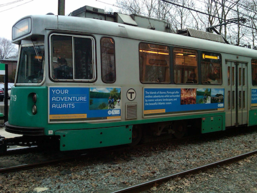
green.png with the image poster.png by applying a homography to the latter.
green.png with the image poster.png by applying a homography to the latter.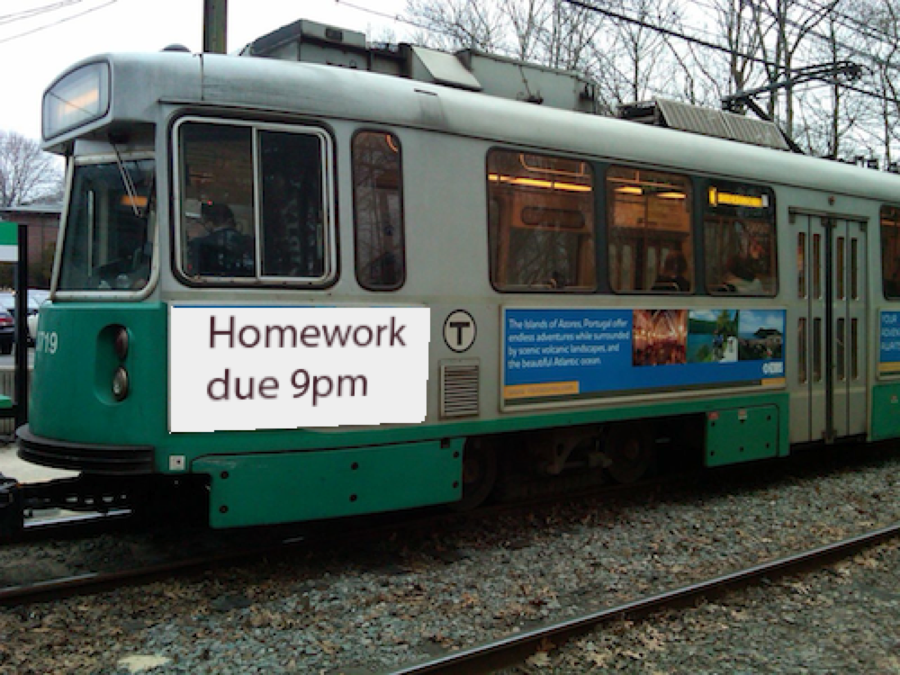
green.png with the image poster.png by applying a homography to the latter.22.8.6 Compute Homography from 4 Pairs of Points⧉
UI. In this section, a user will provide correspondences between two images, by clicking using a patent-pending javascript interface (pano_ui.html), and your job is to infer the homography matrix that maps the 4 points from the first image to the corresponding 4 points in the other image. As in the warping problem set, the user needs to click on points in the same order for the left and right images. When using the UI, you need to select points that are as well spread as possible for the computation to be well conditioned. Specifically, avoid all-collinear points.
Correspondences. The correspondences will be provided as an array of CorrespondencePair, where each CorrespondencePair stores ($x1,y1,z1)$, the coordinates of the point in the first image and ($x2,y2,z2)$, the coordinates in the second. The test function testComputeHomographyPoster in a6_main.cpp gives an example of how to use it.
Homography scaling. A homography matrix is always defined up to a scaling factor. This means that $H$ and $kH$ represent the same geometric transformation for any non-zero scalar $k$. In this assignment, we will use a quick and dirty way to resolve the scale ambiguity and will assume that the bottom right coefficient of the homography is 1. This could create some problems if the true family of matrices $H$ had a zero there, but we will ignore this and leave the cleaner solution based on SVD as extra credit.
Write a function Matrix computeHomography(const CorrespondencePair[4]) that takes a list of 4 point correspondences and returns a $3 \times 3$ homography matrix that maps the first point of each pair to the second point. That is, the homography maps from the first image to the second image.
The details of the algorithm are exposed below.
Outline of Steps.
(a) We would like to solve for the homography that maps 4 points in the first image to the corresponding 4 points in the second image. In general, a homography $H$ correspondence equations can be written:
Where the unknowns are $a, b, c, d, e, f, g, h$, and we know $x, y$ and $x', y'$ for 4 sets of points. $w'$ is not known, but can be deduced easily from other quantities.
(b) You need to create a matrix $A$ and vector $B$ so that the 8 remaining coefficients ( $a, b, c, d, e, f, g, h$) of the homography are encoded in an 8-dimensional vector $x$ that satisfies $Ax=B$.
You have two equations for each pair of corresponding points. To be clear, the $x$ vector in $Ax=B$ is actually $(a, b, c, d, e, f, g, h)^T$.
Do not get confused between the $3 \times 3$ homography matrix and the $8 \times 8$ matrix $A$ for the linear system.
We recommend that you write a subroutine that fills in two rows of the matrix and vector for a given correspondence pair, since the pattern is the same for all pairs of points.
(c) Use the inverse() member function of the Matrix class to compute the inverse of matrix $A$ and multiply it with $B$. You can also have a look at the documentation in Eigen and search for linear system solvers.
(d) Once you have solved the system, reshape your vector $x$ into a $3\times 3$ matrix.
Debugging. Homographies and projective spaces are big scary things. Do not try directly with the provided pairs of points. Use simpler cases. Think about pairs of correspondences where you can compute the matrix easily by hand. Try to infer the identity or a translation. You can also use testComputeHomography in a6_main.cpp to help test your function, it should give you the coefficients from testApplyHomography.
22.8.7 Bounding boxes⧉
In the examples so far, the output image is the same size as one of the two inputs. But for panorama stitching, we want to create a bigger output image that encompasses all points from both images.
For this, we need to compute the size of the final output image. Additionally, the final image might be extended towards the negative coordinates with respect to the reference image. To handle this we will translate the reference, so that the pixel coordinates in the final output start at $(0,0)$.
Transform a bounding box⧉
To compute the required size for one image, we forward-transform its four corners to the output space. We will represent the resulting required size as a bounding box, encoded by its minimum and maximum $x, y$ coordinates.
Be careful: whereas we usually need to consider the inverse warp to go from output coordinates into source ones, here we need to do the opposite and figure out where the bounds of the source project into the output space.
Write a function BoundingBox computeTransformedBBox(int imwidth, int imheight, Matrix H) that takes an image size and a homography as input and returns the BoundingBox of the output coordinates.
Use testComputeTransformedBBox in a6_main.cpp to help test your function. Hint: implementing the optional Image drawBoundingBox(const Image &im, BoundingBox bbox) is useful for debugging bounding boxes.
Bounding box union⧉
When stitching N images, the output is the union of the N bounding boxes.
Write a function BoundingBox bboxUnion(BoundingBox B1, BoundingBox B2) that takes two bounding boxes and returns a bigger bounding box that tightly encompasses the union of the bounding boxes.
Use testBBoxUnion in a6_main.cpp to help test your function.
Translation⧉
After computing and merging the bounding boxes of the N images (including that of the reference), we often will have the situation where the upper-left corner of the bounding box has negative coordinates. This is illustrated in the figure below.
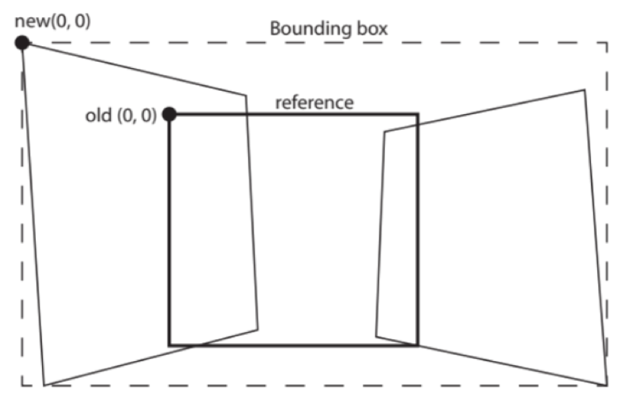
If the upper-left corner of the bounding box has negative coordinates, we need to translate the coordinate system of the reference image to set this corner to coordinates $(0, 0)$. The translation vector is simply the negative of this corner's coordinates. You can then obtain the translation homography matrix for translation by $(t_x t_y)^T$ as:
Write a function Matrix makeTranslation(BoundingBox B) that takes a bounding box as input and returns a $3\times 3$ matrix corresponding to a translation that moves the upper left corner of the bounding box to $(0, 0)$.
Use testTranslate in a6_main.cpp to help test your function.
Putting it all together⧉
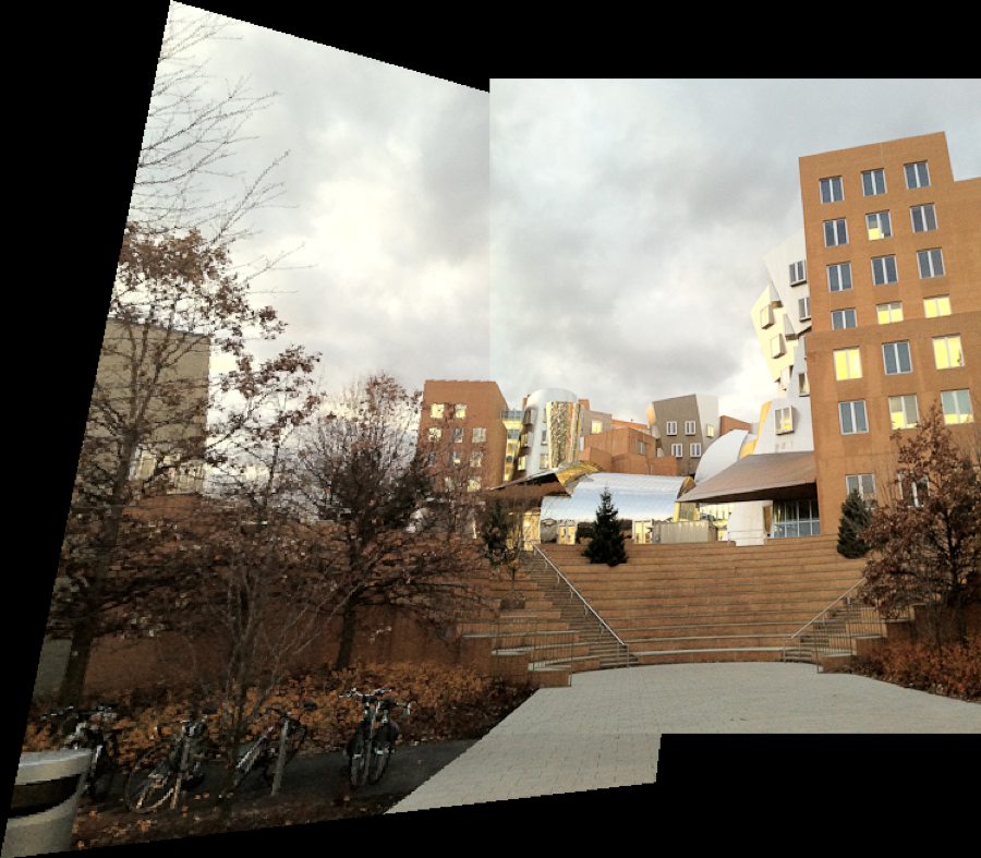
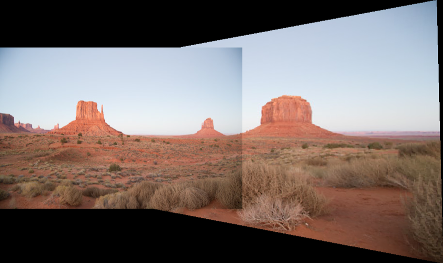
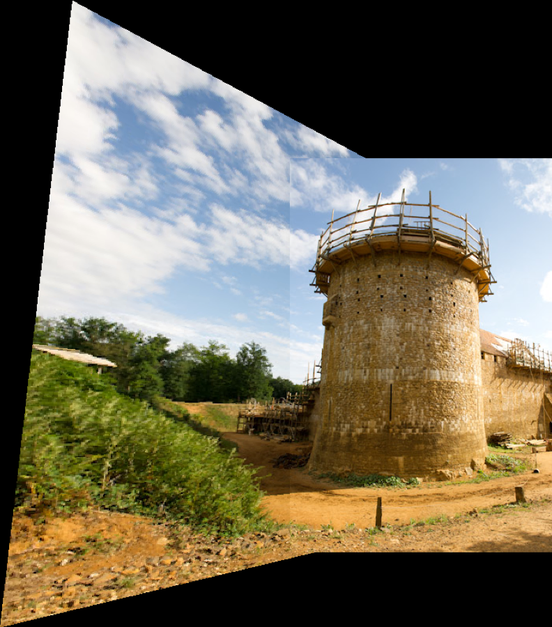
Write a function Image stitch(const Image &im1, const Image &im2, const CorrespondencePair correspondences[4]) that takes two images and their point correspondences and outputs a stitched panorama in the coordinate system of the second (reference) image.
You first need to compute the homography between the two images. Then compute the resulting bounding box and translation matrix. Create a new black image of the size of the bounding box. Then use a combination of your translation and homography matrix to composite both images into the output. Be careful that you also need to transform the second (reference) image to take the translation into account and that you need to combine the translation and the homography for the first image. Use the right matrix product!
Use testStitchStata, testStitchMonu, and testStitchGuedelon in a6_main.cpp to help test your function. See the figure below.
6.8370 only (Or 5% Extra Credit for 6.8371): Speed up Warping using Bounding Boxes⧉
Accelerate the warping function by restricting the warping loop using the bounding box of each image.
Implement void applyhomographyFast(const Image &source, Image &out, Matrix &H, bool bilinear=false). Make sure you see a speed-up of at least 5x for the green and poster example. Use H.inverse() to calculate $H^{-1}$ and clamp = true during interpolation.
Use testApplyHomographyFast in a6_main.cpp to help test your function.
6.8370 only (Or 5% Extra Credit for 6.8371): Extra Test Cases and Images⧉
In homography_extra_tests.h, similar to testStitchStata, write the following test cases: testStitchScience(), to stitch science-1.png and science-2.png; testStitchConvention(), to stitch convention-1.png and convention-2.png; testStitchBoston1(), to stitch boston1-1.png and boston1-2.png.
Create output files science-stitch.png, and convention-stitch.png, and boston1-stitch.png. Please include these images in the zip files, where these three images are directly in the zip file (no extra folders). Use the provided javascript UI to choose the 4 point pairs needed for stitching.
22.8.8 Extra Credit (up to 10% total)⧉
- (5%): Implement a least square estimation of the homography for more than four pairs of points.
- (5%): Apply homography for document rectification (take a picture of a document with text, try to recify so that the text becomes straight and horizontal lines).
- (5%): Estimate the homography with only two pairs of points, assuming the homography is rotation-only.
- (5%) Use SVD to alleviate the assumption that the bottom right coefficient of the homography matrix is 1.
- (5%): Improve the javascript UI.