22.7 Problem Set 5 — Resampling, warping, and morphing⧉
22.7.1 Summary⧉
This problem set has several questions for extra credit. Feel free to attempt them, but do the main problems first. The maximum extra credit is 10%. The last section of this is submitting a photo of yourself, which might take some time depending on what type of person you are. So don't put it off!
- Scaling using nearest-neighbor and bilinear reconstruction
- Scaling using bicubic and Lanczos methods (6.8370 only)
- Image warping according to one pair of segments
- Image warping according to two lists of segments, using weighted warping
- Image morphing
- Take a photo of yourself
22.7.2 Resampling⧉
In this section, we will rescale images, starting with simple transformations and naïve reconstructions. See the figure below for examples of scaling with various methods, together with a small crop of the resulting image to highlight the differences.


scaleNN.
scaleNN (zoom).
scaleLin.
scaleLin (zoom).
Basic Image scaling.
Basic scaling with nearest-neighbor⧉
The first operation we consider is the re-scaling of an image by a global scale factor $s$. If $s > 1$, the operation will enlarge the input. If $0 < s < 1$, it will shrink the input.
To implement this operation, we need to create a new Image object that is $s$ times larger (resp. $\frac{1}{s}\times$ smaller if $s<1$) than the original in both width and height. Use floor() to get an integral size for the new image.
We now have to fill the pixel values of this new image from those of the input: this is called re-sampling. For each pixel in the new image, we look up the color value in the input image at a location that corresponds to the inverse transform (in this case a scaling by $\frac{1}{s}$). In general this location will not be on grid and we'll have to estimate the color at this location using information from the neighboring pixels.
The simplest technique to sample the new value is called nearest-neighbor re-sampling: we round-off the real coordinates to the nearest integers and use the input's color at this new location to be the value of the current output pixel.
1. Implement the
Image scaleNN(const Image &im, float scale)function inbasicImageManipulation.cpp. This function should create a new image that isscaletimes the size of the input using the nearest-neighbor re-sampling method.
Scaling with bilinear interpolation⧉
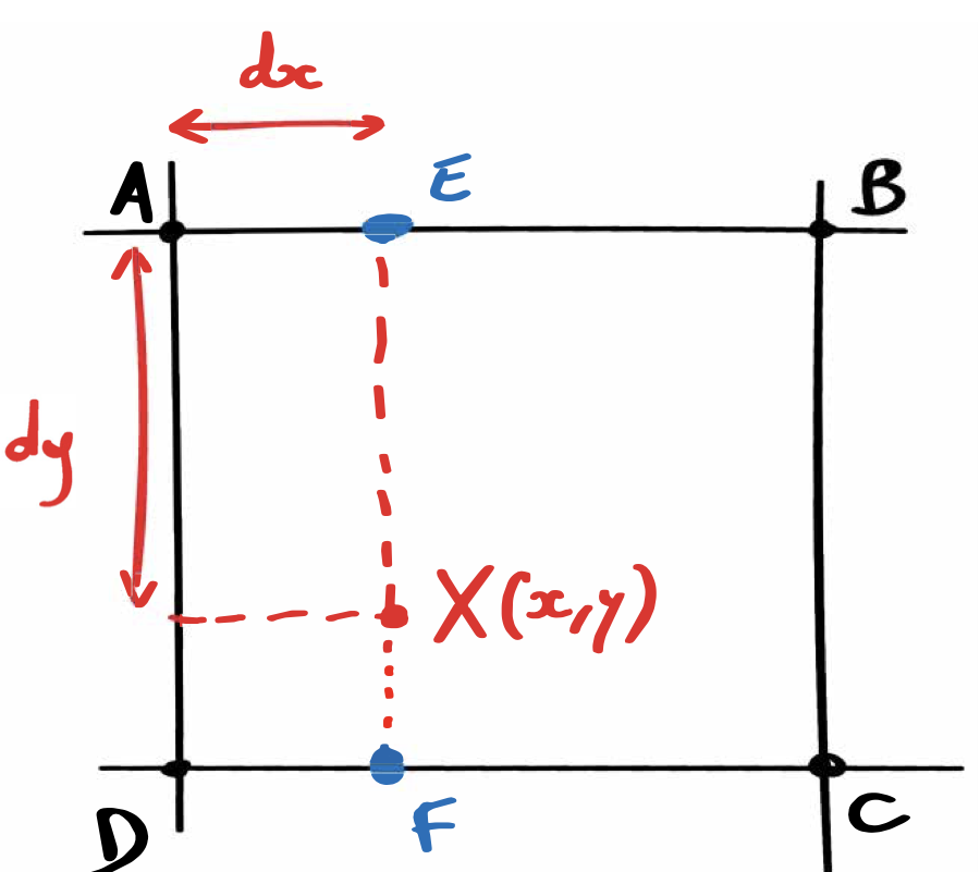
Nearest-neighbor re-sampling creates blocky artifacts and pixelated results. We will address this using a better reconstruction based on bilinear interpolation. For this, we consider the four pixels immediately around the computed real coordinates and perform two linear interpolations. We first linearly interpolate along $x$ the colors of the top and bottom pairs of pixels. Then we interpolate these two values along $y$ to get the final sample. The interpolation weight are driven by the distance from the corners (see the figure below).
2.a Implement
float interpolateLin(const Image &im, float x, float y, int z, bool clamp)inbasicImageManipulation.cpp. This function takes floating point coordinates and performs bilinear reconstruction on the given channelz. Don't forget to use smart accessors to make sure you can handle coordinates outside the image.2.b Next, write an image scaling function
Image scaleLin(const Image &im, float scale)inbasicImageManipulation.cppthat rescale using linear interpolation by callinginterpolateLinwhere appropriate. Useclamp = true.
Bicubic and Lanczos (required for 6.8370, 5% Extra credit for 6.8371)⧉
You can obtain a better interpolation by considering a larger pixel footprint and using smarter weights, such as that given by a bicubic or Lanczos functions.
You may think of resampling from the view point of convolution to better understand how bicubic/Lanczos resampling kernels work. For example, bilinear interpolation for $3\times$ upscaling would be equivalent to first scaling the image naïvely (by only taking the existing pixels from the source image and keeping the rest as blank) and then applying a $5\times 5$ convolution kernel (how does the kernel look like? A square pyramid) to the naïvely scaled image. Hint: This means that an easy implementation of bicubic and Lanczos resampling is to follow the steps of convolution and use analytical weights $k(x)$ instead of numerically discretized ones. And bilinear/bicubic/Lanczos resampling is separable, which means you can multiply horizontal and vertical weights $k(x)$ and $k(y)$ to get the 2D weight.
3. Implement the
Image scaleCubic(const Image &im, float scale, float B, float C)function inbasicImageManipulation.cpp. This function should create a new image that isscaletimes the size of the input using a bicubic filter kernel. We will use the kernel parametrization from Mitchell and Netravali ("Reconstruction Filters in Computer Graphics", Mitchell and Netravali 1988):$$ k(x) = \frac{1}{6}\begin{cases} (12 - 9B - 6C)|x|^3 + \\ (-18 + 12B + 6C)|x|^2 + (6 - 2B) & \text{if } |x| < 1 \\ (-B - 6C)|x|^3 + (6B + 30C)|x|^2 + \\ (-12B - 48C)|x| + (8B + 24C) & \text{if } 1 \leq |x| < 2 \\ 0 & \text{otherwise} \end{cases} $$A nice parameter to test your filter kernel is $B=C=\frac{1}{3}$.
4. Implement the
Image scaleLanczos(const Image &im, float scale, float a)function inbasicImageManipulation.cpp. This function should create a new image that isscaletimes the size of the input using a Lanczos filter kernel. The kernel is:$$ k(x) = \begin{cases} \mathrm{sinc}(x)\,\mathrm{sinc}(x / a) & \text{if } |x| < a \\ 0 & \text{otherwise} \end{cases} $$where $\mathrm{sinc}(x)=\sin(\pi x)/(\pi x)$. A nice parameter to test your filter kernel is $a=3$.
Rotations (5% extra credit)⧉
5. Implement the function
rotate(const Image &im, float theta)inbasicImageManipulation.cppthat rotates an image around its center by $\theta$ radians. Hint: use your bilinear interpolation function and the center position already present in the starter code.
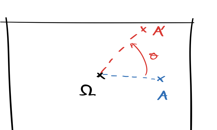
rotate.Rotation with an angle $\theta>0$ with respect to the center of the image (to get the pixel value at $A'$, sample from location $A$ in the input image. Last two images: example rotation by $\frac{\pi}{4}$ using rotate.
22.7.3 Warping and morphing⧉
In what follows, you will implement image warping and morphing according to Beier and Neely's method, which was used for special effects such as those of Michael Jackson's Black or White music video (<https://youtu.be/F2AitTPI5U0>).
We highly recommend that you read the provided original article, which is well written and includes important references such as Ghost Busters.
Beier, Thaddeus, and Shawn Neely. "Feature-based image metamorphosis." ACM SIGGRAPH Computer Graphics. Vol. 26. No. 2. ACM, 1992.
The full method for warping and morphing includes a number of technical components and it is critical that you debug them as you implement each individual one. A copy of the paper is included in the handout.
Basic Vector Tools⧉
Warping and morphing geometrically distort an input image. This requires a few vector operation which you'll implement. We provide you a basic Vec2f class to represent 2D vectors.
6.a In
morphing.cpp, implementVec2f operator+(const Vec2f & a, const Vec2f & b)to sum two vectors $\textbf{a}+\textbf{b}$.6.b In
morphing.cpp, implementVec2f operator-(const Vec2f & a, const Vec2f & b)that returns the difference $\textbf{a}-\textbf{b}$.6.c In
morphing.cpp, implementVec2f operator*(const Vec2f & a, float f)that implements multiplication by a scalar $f\cdot \textbf{a}$.6.d In
morphing.cpp, implementVec2f operator/(const Vec2f & a, float f)that implements division by a scalar $\textbf{a} / f$.6.e In
morphing.cpp, implementVec2f dot(const Vec2f &a, const Vec2f &b)that implements the dot product of two vectors: $a_x * b_x + a_y * b_y$.6.f In
morphing.cpp, implementfloat length(const Vec2f &a)that returns the length of a vector (in the $L^2$ sense): $\|\textbf{a}\| = \sqrt{a_x^2+a_y^2}$.6.g In
morphing.cpp, implementVec2f perpendicular(const Vec2f &a)that returns a vector that is perpendicular to a. Hint: either of the two possible directions is fine.
Don't forget to test your functions. We have provided some basic tests for you in a5_main.
Segments⧉
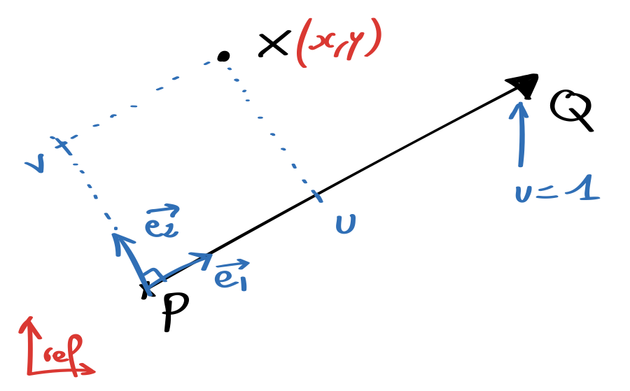
Now that we have some basic tools, we will implement the Segment class, which is critical to Beier and Neely's warping. A Segment represents a directed line segment $\overrightarrow{PQ}$. The class holds a copy of the endpoints $P$ and $Q$, the length of the segment $\|\overrightarrow{PQ}\|$, and a local orthonormal frame $(\overrightarrow{e_1},\overrightarrow{e_2})$. We define:
$\overrightarrow{e_2}$ completes the orthonormal frame (e.g. $\overrightarrow{e_2}$ is perpendicular to $\overrightarrow{e_1}$), see the figure below. Both frame vectors and the length of the segment need to be initialized in the class constructor and can be used directly in its class functions.
7. In
morphing.cpp, complete the constructorSegment::Segment(Vec2f P_, Vec2f Q_)that creates a segment from its two endpoints and initializes the data structure properly.
Now that our Segment class is usable let's implement methods to convert from the global $(x,y)$ coordinates of a point to the local $(u,v)$ coordinates in the reference frame as in Beier and Neely, e.g., equations (1) and (2) in the paper, and the reverse (equation (3)). A word of caution: although $v$ exactly corresponds to the second coordinate in the local frame, $u$ is actually rescaled (so read equation (1) carefully).
8.a Implement
Vec2f Segment::XtoUV(Vec2f &X)to compute the $(u,v)$ coordinates of a 2D point $X=(x,y)$ with respect to a segment as described in the paper.8.b Conversely, implement
Vec2f Segment::UVtoX(Vec2f &uv)to compute the $(x,y)$ global coordinates of a 2D point from its local $(u,v)$ coordinates.8.c Implement the point to segment distance function
float Segment::distance(Vec2f X)as described in section 3.3 of the paper.
Test these methods thoroughly as they will be used in the warping and morphing functions in the later part of the problem set. The function testSegment in a4_main.cpp is great place to write simple test cases.
Warping according to one pair of segments⧉
Now that we have a functional Segment class and an interface to specify line segments, let the fun begin. The core component to warp images is a method to transform an image according to the displacement of a segment.
9. Implement
Image warpBy1(const Image &im, Segment segBefore, Segment segAfter). This is a resampling function that warps an entire image according to one a pair of segments. Hint: Figure 1 of the Beier and Neely paper might be helpful here.
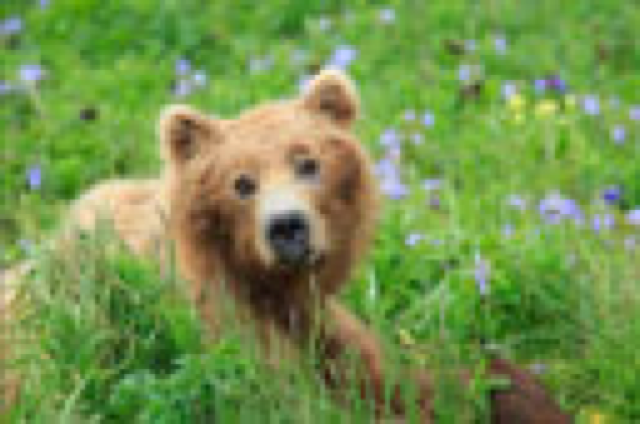
bear.png input image.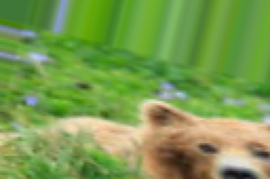
warpBy1 on bear.png.Example output of the warpBy1 function on the bear.png image using segments: before = Segment((0,0), (10,0)) and after = Segment((10, 10), (30, 15)).
The output should be an image of the same size as the input such that the feature under segBefore is now at the location of segAfter. Use bilinear reconstruction (with clamp = true). Again, use simple examples to test this function, see the figure above. Once you are done with this, you have completed the hardest part of the assignment.
Warping according to multiple pairs of segments⧉
In this question, you will extend you warp code to perform transformations according to multiple pairs of segments. For each pixel, transform its 2D coordinates according to each pair of segments and take a weighted average according to the length of each segment and the distance of the pixel to the segments. Specifically, the weight is given according to Beier and Neely:
where $a, b, p$ are parameters that control the interpolation. In our test, we have used $b=p=1$ and $a=10$ (roughly 5% of the image size).
10.a Implement
float Segment::weight(Vec2f &X, float a, float b, float p)based on the formula above.10.b Implement
Image warp(const Image &im, const &vector<Segment> src_segs, const &vector<Segment> dst_segs, float a=10.0, float b=1.0, p=1.0)which returns a new warped image according to the list of before and after segments. Pay attention to the order of the segments, where you should loop over output pixels. Hint: section 3.3 of the paper and the above function will be helpful here.
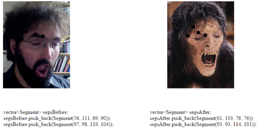
Use the provided javascript UI to specify segments. The points must be entered in the same order on the left and right image. You can then copy-paste the C++ code generated below the images to create the corresponding segment objects.
UI⧉
We provide you with a rudimentary (to say the least) interface to specify segment location from a web browser. It is based on javascript and the raphael library (http://raphaeljs.com/), and improved by students throughout the years. You specify two input images in morph_ui.html (the images must be the same size).
You must click on the segment endpoints in the same order on the left and on the right. Unfortunately, you cannot edit the locations after you have clicked, but you can delete edges by double clicking on them. Once you are done, simply copy the C++ code below each image into your main function to create the corresponding segments.
Morphing⧉
Given your warping code, we will write a function that generates a morph sequence between two images. Again, make sure you are familiar with morphing from the article.
You are given the source and target images, and a list of segments for each image (the position in the list defines the corresponding pairs of segments, so the lists should have the same number of elements). You must generate $N$ images morphing from the first input image to the second input image.
For each image, compute its corresponding time fraction $t$. Then linearly interpolate the position of each segment's endpoints according to $t$, where $t=0$ corresponds to the position in the first image and $t=1$ is the position in the last image. You might want to visualize the results for debugging.
You now need to warp both the first and last image so that their segment locations are moved to the segment location at $t$, which will align the features of the images. We suggest that you write these two images to disk and verify that the images align and that, as $t$ increases, the images get warped from the configuration of the first image all the way to that of the last one.
Finally, for each $t$, perform a linear interpolation between the pixel values of the two warped images.
Your function should return a sequence of images. For debugging you can use your main function to write your images to disk using a sequence of names such as morph_1.png, morph_2.png, …, see testMorph in a5_main.cpp.
11. Implement
morph(im0, im1, listSegmentsBefore, listSegmentsAfter, N=1, a=10.0, b=1.0, p=1.0). It should return a sequence of $N$ images in addition to the two inputs (i.e., when called with the default value of 1, it only generates one new image for $t=0.5$). The function should check thatim0andim1have the same size, and throw an exception if not. Note that the interpolation weight should be at the scale of $[0,1]$, so we need a time constant of $1/(N+1)$ here.
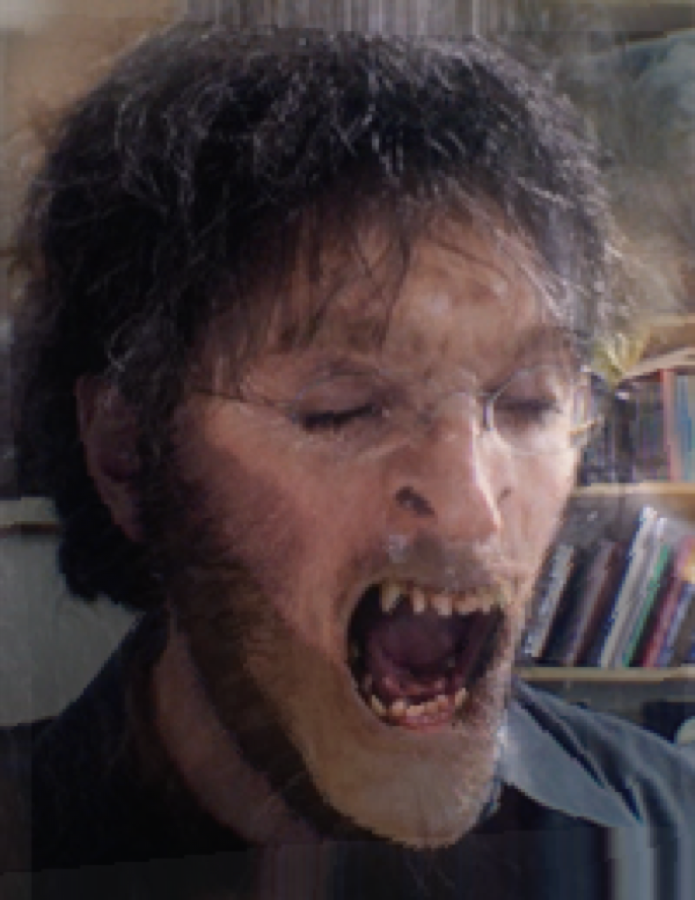
Morph example. Your morphs will look slightly different depending on what segments you use.
Visualize Results. Aside from just looking at the images, you can explore your results at <https://www.mit.edu/~adalca/tipiX/> if you wish. Click on load and load your morphed images (make sure to respect the required naming). Then explore your results using the pointer, or click "play" from the top-right information panel.
There are several ways to make a video (or a .gif) out of your files (note this is not required). You can install ffmpeg http://ffmpeg.org/ but this involves some number of dependencies. Then use it with, e.g. ffmpeg -i tes_morph_%02d.png out.gif.
Class morph⧉
We'll use the code implemented in this problem set to create a class morph. In order to do that, we need a photo of your face.
12. Submit a selfie (of yourself) as a PNG file named
myface.pngin theInputfolder of your submission. Feel free to make a silly face if you want. Make sure it's named correctly and in the right folder so that our script can pick up your image.
Make sure your photo follows the following specifications:
- 500 x 600 (500 width, 600 height). There are image rescaling tools online, or you can use what you implemented earlier this pset!
- The background must be a single color of either white or otherwise pale color, and there shouldn't be clutter in your background.
- Your entire face (everything from the neck up) should be visible. Think passport photo.
- The file should be a png. If it is not, there should be plenty of conversion tools online.
In the next pset, we will ask you to run your morphing code from your own face to the face of a peer. Get excited!
22.7.4 Extra credit⧉
Here are ideas for extensions you could attempt, for 5% each. At most, on the entire assignment, you can get 10% of extra credit:
- Improve the javascript UI. The amount of extra credit you get is dependent on how much improvement you make. We may also keep your improvements for future classes!
- Extend to movies, where segments are specified at a number of keyframes.
- Morphable face models (see <https://www.face-rec.org/algorithms/3D_Morph/morphmod2.pdf>. Data is at <https://github.com/3d-morphable-models/curated-list-of-awesome-3D-Morphable-Model-software-and-data>)