22.5 Problem Set 3 — Denoising and demosaicking⧉
22.5.1 Summary⧉
- Denoising based on averaging
- Variance and signal-to-noise computation
- Image alignment using brute force least squares
- Basic green channel demosaicking
- Basic red and blue channel demosaicking
- Edge-based green channel demoasaicking
- Red and blue channel demosaicking based on difference to green
- 6.865 only: reconstructing the color of old Russian photographs
22.5.2 Denoising from a sequence of images⧉
Basic sequence denoising⧉
In our image formation model, the image captured by the camera $I(x,y,z)$ is the sum of a latent (i.e. unknown) image $\hat{I}(x,y,z)$ and some random noise $n(x,y,z)$:
Note that both $n$ and $I$ are random variables in this model. If we further assume that $n$ is zero-mean, then the expected value $\mathbb{E}(I)=\hat{I}$ is the true image we wish to capture.
This gives us a simple denoising method: we can take $N$ shots of the same subject (i.e. the subject and the camera are static) and average these measurements (i.e. the captured images). The empirical mean is an estimate of the true image $\hat{I}$:
In the equation above $I_k$ is a realization of the random variable $I$.
- Write a simple denoising method
Image denoiseSeq(const vector<Image> &imgs)inalign.cppthat takes an image sequence as input and returns a denoised version by computing the per-pixel average of all the images. Note: at this point, you should assume that the images are perfectly aligned and have the same size.
Try your function on the sequence in the directory aligned-ISO3200 following the example in a3_main.cpp. We suggest testing with at least 16 images and experimenting with more images to see how well the method converges.
ISO⧉
The Inputs folder contains two image sequences, aligned-ISO400 and aligned-ISO3200. The scene is identical for both sequences, but camera settings differ
- The ISO400 sequence was captured with long exposure and only moderate electronic amplification (higher ISO means more amplification) of the sensor readout.
- For the ISO3200 sequence, the exposure time was reduced by a factor of 8. To make both sequences appear equally bright despite the shorter exposure time, ISO was increased by a factor of 8.
- Denoise both the ISO400 sequence and the ISO3200 sequence. Compare the results. Do they match your expectations? (Answer in the submission system)
Variance⧉
Given the same set of $N$ measurements (each measurement being an entire image), we compute the variance as:
We can then use the variance to get an estimate of the noise level in the image. We'll compute the log signal-to-noise ratio as:
A useful summary statistic is the peak-signal-to-noise ratio (PSNR) which is the maximum value of of the SNR (or log SNR).
3.
- 3.a Write a function
Image logSNR(const vector<Image> &imSeq, float scale=1.0/20.0)inalign.cppthat returns an image visualizing the per-channel per-pixel log signal-to-noise ratio (using the formula above) scaled byscale. Note: In the SNR computation, for 'numerical lubrication,' add a small value ($10^{-6}$) to the denominator to avoid division by zero.- 3.b Compare the signal-to-noise ratio of the
ISO 3200andISO 400sequences. Which ISO has better SNR? Answer the question in the submission system.
To get a more reliable estimate in the SNR use at least 16 images, (more will give you better estimates). Visualize the variance of the images in aligned-ISO3200 in a3_main.cpp.
Alignment⧉
The image sequences you have looked at so far have been perfectly aligned. Sometimes, the camera might move, so we need to align the images before denoising. In what follows we will assume that the misalignment is only horizontal or vertical translation on the image plane.
4.
- 4.a Write a function
vector<int> align(const Image &im1, const Image &im2, int maxOffset=20)inalign.cppthat returns the horizontal and vertical offset (e.g. [x,y]) that best alignsim2to matchim1.To align the images, use a brute force approach that tries every possible integer translation (in the range [-
maxOffset,maxOffset] in each direction) and evaluates the quality of a match using the the sum of the squared pixel differences. Ignore pixels that are within distance ofmaxOffsetfrom the image boundaries in the computation of the cost to avoid edge issues.You may want to use
float Image::smartAccessor(int x, int y, int z, bool clamp)to clamp pixel values that are outside of the image bounds.Make sure to test your procedure before moving on. A simple test would be to generate two image, say $100 \times 100 \times 1$ and have one contain a white rectangle at $[40, 40] \rightarrow [60, 50]$ and the other at $[50, 60] \rightarrow [70, 70]$ and test your method using $\mathtt{maxOffset} = 20$.
- 4.b Use
alignto create a functionImage alignAndDenoise(const vector<Image> &imSeq, int maxOffset=10)inalign.cppthat aligns all images to the first image in the sequence then outputs a denoised image. This allows you to produce a denoised image even when the input sequence is not perfectly registered to begin with. RunningalignAndDenoisecan take a few minutes.
Use the images in the folder Input/green/noise-small-<xx>.png where $\mathtt{xx} = [1,18]$ to test your procedure and replicate the results of the denoising figure below.
5.
- 5.a What
maxOffsetdid you use? Qualitatively, what image features are preserved? Which are eliminated? What else can you think of doing to reduce the noise in these images ? (Answer in the submission form).
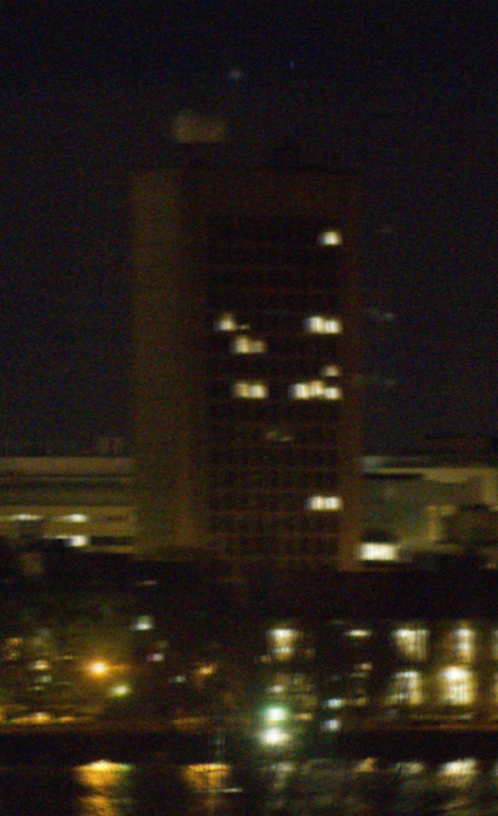
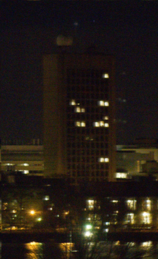
Result of denoising the first 9 images of the green sequence (a) naively averaging and (b) averaging after first aligning the images. Zoom in on the image edges, what do you notice?
22.5.3 Demosaicing⧉
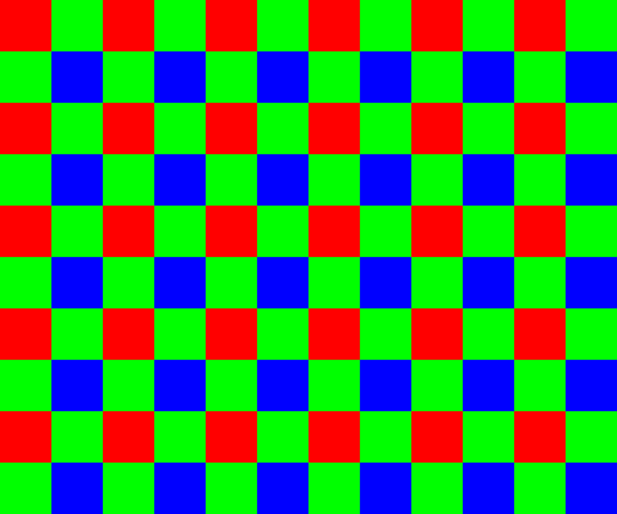
Most digital sensors record color images through a Bayer mosaic, where each pixels captures only one of the three color channels. Subsequently, software interpolation is then needed to reconstruct all three channels at each pixel. The green channel is recorded twice as densely as red and blue, as shown in the Bayer mosaic figure above.
- Why does it make sense to oversample the green channel compared to red and blue? (Answer in the submission form.)
We have provided a number of raw images for you in the folder Input/raw. These raw images are encoded as greyscale images. You can open them in your favorite image viewer and zoom in to see the pattern of the Bayer mosaic.
Your task in what follows is to write functions to demosaic them. We encourage you to debug your code using signs-small.png because it is not too large and exhibits many of the interesting challenges of demosaicing.
For simplicity, we will ignore the case of pixels near the image boundaries. That is, the first and last rows (and columns) of pixels don't need to be reconstructed. This will allow you to focus on the general case and not worry about whether neighboring values are unavailable. It's actually not uncommon for cameras and software to return a slightly-cropped image for similar reasons (<http://www.luminous-landscape.com/contents/DNG-Recover-Edges.shtml>);
Basic green channel⧉
We will begin with the green channel since it contains more observed pixels.
- Write a function
Image basicGreen(const Image &raw, int offset)indemosaic.cppthat takes as input a raw single-channel grayscale image and returns a single-channel 2D image corresponding to the interpolated green channel. Note: when you are testing, keep in mind that our Image class reads grayscale png images as a three-channel image where all channels have the same content.The offset encodes whether the top-left pixel or its neighbor immediately to the right is the first green pixel (possible values are $[0,1]$). Make your code general so that it works for either offset since different cameras use different conventions. In the case of the Bayer mosaic figure, the second pixel in the first row is green
offset=1. For the imagesigns-small.pngoffset=1. Hint: notice that the starting point varies, but the structure of the pattern is fixed.For pixels where green is recorded, simply copy the value. For unobserved pixel, fill in the green value as the average of its 4 recorded green neighbors (up, down, left, right).
For simplicity, do not attempt to interpolate the first and last row and column of the image. Just copy their pixel values from the raw image into your output. By ignoring the reconstruction of these rows and columns all the pixels you need to reconstruct have a 4-neighborhood.
Try your image on the included raw files and verify that you get a nice smooth interpolation. You can try on your own raw images by converting them using the program dcraw.
Basic red and blue⧉
So far we have obtained our demosaic green channel. Now we will be applying a similar process to the remaining red and blue channels. Since the sampling frequency of these channels is the same, we will treat them as equivalent.
8.
- 8.a Write a function
Image basicRorB(const Image &raw, int offsetX, int offsetY)indemosaic.cppto deal with the sparser red and blue channels. The function takes a raw image and returns a 2D single-channel image as output. The inputoffsetX, offsetYare the coordinates of the first pixel of the channel we are demosaicing (hint: as before the starting location of the pattern varies but the structure does not). In the case of the Bayer mosaic figure, the red channel begins at pixel (0, 0), and the blue channel at (1,1). That is to extract the red and blue channel we would call the function twice as:Image red = basicRorB(raw, 0, 0);Image blue = basicRorB(raw, 1, 1);Similar to the green-channel case, copy the values when they are available. For unknown pixels that have two direct neighbors that are known (left-right or up-down), simply take the average between the two values. For the remaining case, interpolate the four diagonal pixels. You can ignore the first and last two rows (or columns) to make sure that all unknown pixels have the necessary neighbors.
- 8.b Implement a function
Image basicDemosaic(const Image &raw, int offsetGreen=1, int offsetRedX=1, int offsetRedY=1, int offsetBlueX=0, int offsetBlueY=0)indemosaic.cppthat takes a raw image and returns a full three-channel RGB image demosaiced with the above functions. You might observe some checkerboard artifacts around strong edges. This is expected from such a naïve approach.
Try your basicDemosaic function on other images in the Input/raw/ folder. We will leave it up to you to figure out the offsets for other images (if any).
22.5.4 Edge-based green⧉
One central idea to improve demosaicing is to exploit structures and patterns in natural images. In particular, structures like edges can be exploited to remove artifact from the naive interpolation. The intuition is to limit the interpolation to regions where pixel values are expected to be similar and compute the value of unobserved pixels based on observed pixels in the same regions.
We will implement the simplest version of this principle, 'edge-based demosaicing', to improve the interpolation of the green channel (we focus on green because it has a higher sampling rate). In edge-based demosaicing, we will compute the values of unobserved pixels based on the values of neighbors from the same region, where regions are determined by pixels being on the same side of an edge. We will focus on only two types of edges: horizontal and vertical. To compute these edges, we rely on pixel differences of the top-bottom neighbors (or left-right neighbors) of the unobserved pixel. Based on the value of these 'edges' we will decide which of the two neighbor pairs to average to obtain the final value of our unobserved pixel. The final value for an unobserved pixel will be the average of only two pixels, either up and down or left and right based on the values of the edges.
9.
- 9.a Should we interpolate along the direction of biggest or smallest variation in pixel values? (Answer in the submission form.) Hint: it is up to you to think or experiment and decide what to do. It's also possible that the slides might help…
- 9.b Write a function
Image edgeBasedGreen(const Image &raw, int offset=0)indemosaic.cppthat takes a raw image and outputs an adaptively interpolated single-channel image corresponding to the green channel. Aside from the adaptive components, all other aspects are the same asbasicGreen. Hint: this function should give better results for horizontal and vertical edges than its basic counterpart.- 9.c Write a function
Image edgeBasedGreenDemosaic(const Image &raw, int offsetGreen=1, int offsetRedX=1, int offsetRedY=1, int offsetBlueX=0, int offsetBlueY=0)indemosaic.cppthat takes a raw image and returns a full RGB images with the green channel demosaiced withedgeBasedGreenand the red and blue channels demosaiced withbasicRorB.- 9.d Do you see any artifact with this new edgeBased method? If yes, what could be improved? (Answer in the submission form.)
22.5.5 Red and blue based on green⧉
A number of demosaicing techniques work in two steps. First they focus on getting a high-resolution interpolation of the green channel using a technique such as edgeBasedGreen. Then they rely on this high-quality green channel to guide the interpolation of the red and blue channels.
One simple such approach is to interpolate the difference between red and green channel. That is, instead of interpolating the red channel directly, we interpolate the difference between red and green channel of the observed neighboring pixels and add the missing value from green channel after interpolation. The same procedure holds when applied to the blue channel.
10.
- 10.a Write a function called
Image greenBasedRorB(const Image &raw, Image &green, int offsetX, int offsetY)indemosaic.cppthat interpolates the red (or blue) channels as the difference R-G (or B-G).In this case, we are not trying to be clever about 1D structures because we assume that this has been taken care of by the green channel. Aside from the interpolation differences, this function is identical to its basic counterpart
basicRorB.
- 10.b Write a function
Image improvedDemosaic(const Image &raw, int offsetGreen, int offsetRedX, int offsetRedY, int offsetBlueX, int offsetBlueY)indemosaic.cppthat takes a raw image and returns a full RGB images with the green channel demosaiced withedgeBasedGreenand the red and blue channels demosaiced withgreenBasedRorB.
Try this new improved demosaicing pipeline on signs-small.png to replicate the results of the demosaicing figure below. Notice that most (but not all) artifacts are gone.

basicDemosaic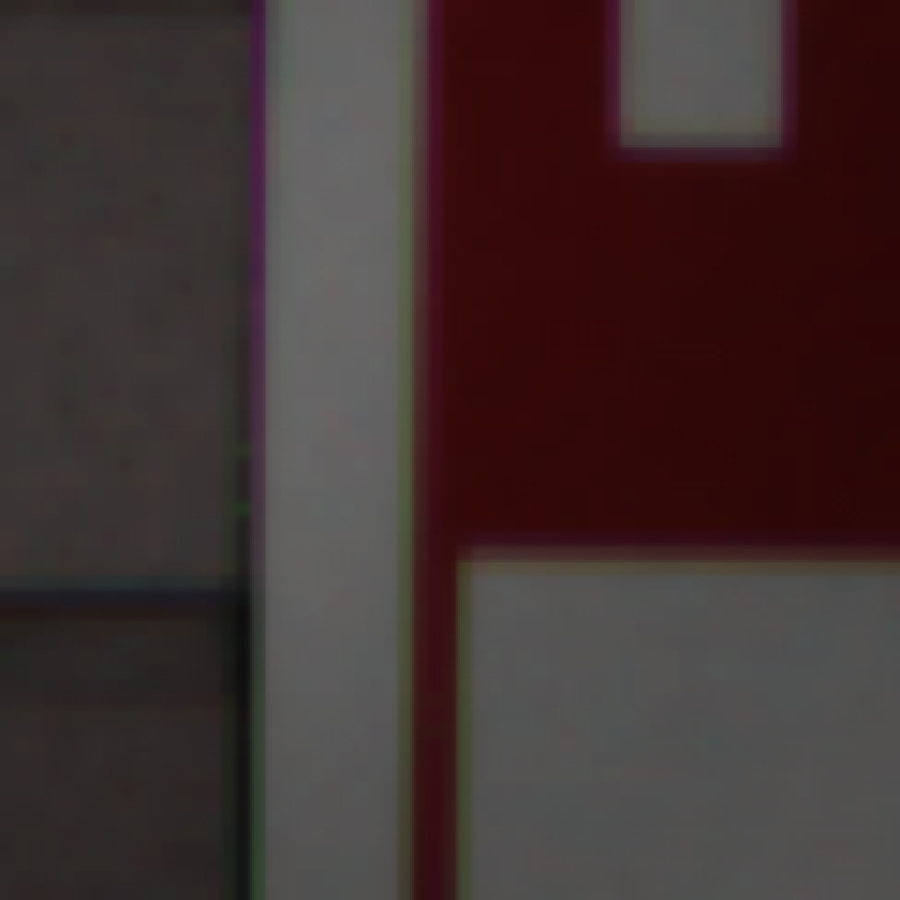
edgeBasedGreenDemosaic
improvedDemosaicResults of demosaicing using the 3 different methods. Notice how artifacts appear around the edges of the resulting image when using basic interpolation. However, an edge aware demosaicing algorithm significantly decreases the artifacts in these regions.
22.5.6 6.865 only (or 5% Extra Credit): Sergey Prokudin-Gorsky⧉
The Russian photographer Sergey Prokudin-Gorsky took beautiful color photographs in the early 1900s by sequentially exposing three plates with three different filters: <http://en.wikipedia.org/wiki/Prokudin-Gorskii> <http://www.loc.gov/exhibits/empire/gorskii.html>.
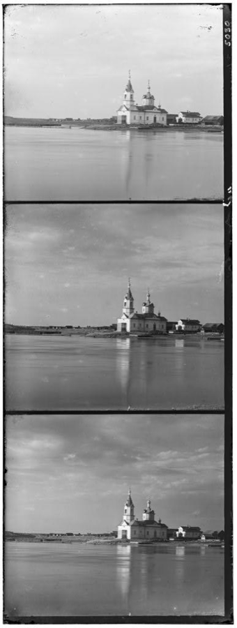
We include a number of these triplets of images in Input/Sergey (courtesy of Alyosha Efros). Your task is to reconstruct RGB images given these inputs. In order to do so, we will first split the triplets then align them.
Cropping and splitting⧉
- Write a function
Image split(const Image &sergeyImg)inalign.cppthat vertically splits an image into 3 segments and turns returns the segments as a single 3-channel image. Note that the input triplet order from top to bottom is blue, green, red, and you are supposed to output a RGB image.We have cropped the original images so that the image boundaries are approximately 1/3 and 2/3 along the y dimension. Use
floorto compute the height of your final output image from the height of your input image.
Alignment⧉
The image that you get out of your split function will have its 3 channels misaligned. Use the align function to correct this misalignment.
- Write the function
Image sergeyRGB(const Image &sergeyImg, int maxOffset=20)inalign.cppthat first calls yoursplitfunction, but then aligns the green and blue channels of your RGB image to the red channel. Your function should return a beautifully aligned color image.
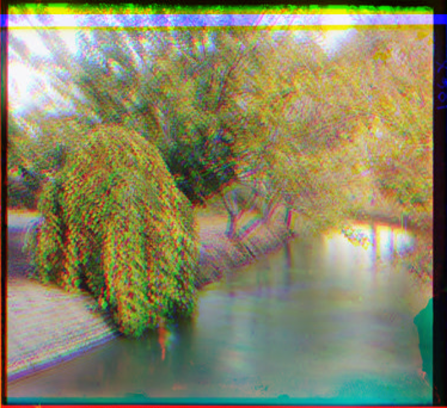
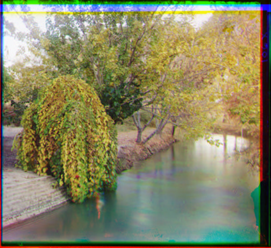
Generating an RGB image from a single grayscale Sergey image
22.5.7 Extra credit (maximum of 10%)⧉
- Speed up the alignment while maintaining accuracy.
- Numerically compute the convergence rate of the error for the sequence denoising at each pixel. Use a regression in the log domain (log error vs. log number of images).
- Implement a coarse-to-fine alignment. Use an image pyramid: <https://en.wikipedia.org/wiki/Pyramid_(image_processing)>
- Take potential rotations into account for alignment. This could be slow!
- Implement smarter demosaicing. Make sure you describe what you did. For example, you can use all three channels and a bigger neighborhood to decide the interpolation direction.
- Use deep learning for denoising or demosaicing (denoising is probably easier in terms of dataset collection)
- Perform demosaicing in 8-bit (e.g. assume the input are integer values [0,255] and perform all operations as integer arithmetic. The goal here is to simulate low-powered image processing hardware. You will have to implement an 8-bit version of the Image class.)