5.2 Bilateral filtering⧉
PS2 implements the bilateral filter (with a YUV chroma variant). → Problem sets (appendix).
A Gaussian blur asks a single question of every neighbour: how close are you? A nearby pixel counts for a lot, a distant one for little, and that is the entire policy. Inside the flat interior of a region that is exactly right. At an edge it is exactly wrong: the blur reaches across the boundary and averages two things that have nothing to do with each other — the bright sky and the dark mountain it sits against. This chapter builds the standard cure, the bilateral filter, which adds a second question to the average: not only how close is this neighbour? but how similar in value is it? That second question — read off the value difference between two pixels — is an affinity, a measure of how much two pixels belong together, and it turns out to be the organizing idea behind an entire family of edge-aware methods. We meet the bilateral first as the remedy for one specific, ugly artefact, and then follow its affinity through cross/joint filtering, the bilateral grid, and a learned grid (HDRnet).
5.2.1 Motivation — local tone-mapping haloes⧉
Start where the bilateral filter earns its keep in this book: tone mapping a high dynamic range (HDR) image. A real scene spans a contrast far larger than any screen or print can reproduce — a sunlit window and the shadowed room behind it can differ by thousands to one — so we must compress the range while keeping the picture legible. The move that works is a two-scale decomposition: split the image into a large-scale base layer (the overall distribution of light — where it is bright, where it is dark) and a fine-scale detail layer (texture, small edges, the fine print), then crush the base hard, leave the detail alone, and recombine. It is the best-of-both trick (Style Reference rule 5): squeeze the part of the signal that carries the offending range, keep the part that carries the look. For HDR we run all of this on log luminance, because the eye reads contrast multiplicatively — a fixed ratio of light should map to a fixed step.
The obvious way to extract the base layer is the tool we already own: a Gaussian blur. Blur the log-luminance image with a wide Gaussian and what survives is the slow, large-scale variation; the detail is whatever the blur threw away. In the flat interior of a region this works beautifully. At a strong edge it fails, visibly and spectacularly.
Picture a bright sky meeting a dark mountain silhouette. The Gaussian base layer is a weighted average of the neighbourhood, and right at the silhouette that neighbourhood straddles the boundary: the blur pulls bright sky values onto the dark side of the edge and dark mountain values onto the bright side. The base no longer respects the edge — it ramps smoothly across it. Compress that base, add the detail back, and the mismatch surfaces as an overshoot: a bright fringe glowing on the dark side of the silhouette, a dark fringe on the bright side. That glowing fringe hugging every high-contrast edge is the classic halo, the signature artefact of naive local tone mapping (Figure 5.2.1).

What we want is a base layer that is smooth within a region but does not average across the boundary into the next region — a filter that blurs everywhere except where the image has a real edge. That is precisely an edge-preserving filter, and the bilateral is the canonical one.
The halo is the cleanest motivation, but far from the only one. The same wish — do not let the filter bleed past an edge — turns up all over computational photography. Denoise a portrait and you want the grain gone from the cheek without the eyelashes smearing into the skin. Stylize or abstract an image and you want flat, poster-like regions with the boundaries kept crisp. Build a selection mask and you want it to snap to edges, not slop across them. These are the same request, served by the same machinery (cross-link to #Compositing, segmentation and matting and to stylization / non-photorealistic rendering (NPR)).
5.2.2 Bilateral filter⧉
Begin from what we already know (name-then-use). A Gaussian blur replaces each pixel with a weighted average of its neighbours, the weight being a spatial Gaussian $g_s(\lVert p - q\rVert)$ of the distance between the centre pixel $p$ and a neighbour $q$: nearby pixels count for a lot, distant ones taper off. It is easiest to watch this on a 1-D scanline — a single row of the image — where the picture becomes a wiggly curve of value against position (Figure 5.2.2).
The trouble, once more, is the edge. A step edge on the scanline — values low on the left, high on the right — gets smeared by the Gaussian, because right at the step the averaging window reaches across the boundary and blends the two plateaus together. This is exactly the bleed that built the halo, seen one dimension down.
The fix is a single extra factor. Keep the spatial Gaussian, but multiply in a second Gaussian — this one on the value difference between the centre pixel and the neighbour, $g_r(\lvert I_p - I_q\rvert)$. This range weight asks "are these two pixels similar in value?" and down-weights neighbours that are too different. A neighbour that is close in space but far in value — one living on the other side of an edge — now earns a weight near zero, however spatially near it sits. The filter, all by itself, declines to average across the edge.
Putting the two Gaussians together gives the bilateral filter (Tomasi & Manduchi 1998). The weight a neighbour $q$ receives at pixel $p$ is the product of the spatial and range terms,
and the output is the normalized weighted average of the neighbours,
Read it back in words (Style Reference rule 3): "average my neighbours, but only those that are both nearby and similar to me." The two widths do different jobs. $\sigma_s$, in pixels, sets how large a region we pool over — the reach of the spatial Gaussian. $\sigma_r$, in intensity units, sets how different is "too different" — the value gap beyond which a neighbour stops counting. Because $\sigma_r$ is measured in the same units as $I$, we must fix the encoding before we can quote it: for HDR tone mapping the filter runs on log luminance (Durand & Dorsey 2002, where a range $\sigma_r \approx 0.4$ in $\log_{10}$ is typical); for ordinary edits it runs on gamma values.
As code, the brute-force bilateral is a double loop with a per-pixel normalization, and one subtlety distinguishes it from convolution: you may precompute the spatial weight $g_s$ (it is the same window everywhere), but the range weight $g_r$ must be recomputed for every pair, because it depends on the value difference at that pixel — so it cannot be tabulated or reused from your Gaussian-blur code. Truncate only the spatial Gaussian to a finite window.
precompute g_s over the window          # spatial weights, same for every pixel
for each output pixel p:
    sum ← 0;  W ← 0                      # accumulator and normalizer
    for each neighbour q in the window around p:
        w ← g_s(‖p − q‖) · g_r(|I[p] − I[q]|)   # range term recomputed per pair
        sum ← sum + w · I[q]
        W   ← W + w
    I_bf[p] ← sum / W                    # per-pixel normalization
For a color image the range distance $|I_p - I_q|$ is the 3-D distance in RGB (or YUV); everything else is unchanged.
Two extreme settings of the range width $\sigma_r$ give two predictable outcomes that bracket the whole filter — the fastest way to sanity-check an implementation (the recipe also lives in Developing, testing & debugging). Figure 5.2.7
- Crank $\sigma_r$ very large. The range term flattens, $g_r \to 1$, and drops out of the product. The bilateral must collapse to a plain Gaussian — so run it side by side with your already-tested Gaussian blur; they should agree pixel for pixel.
- Shrink $\sigma_r$ very small. Now a pixel averages only with near-identical neighbours, so edges stay untouched and the output is essentially the input. Run it on a synthetic half-plane or rectangle (one hard edge): the bilateral must leave that edge razor-sharp.
If either limit misbehaves, the bug is in the range term or the normalization — fix that before trusting any middle $\sigma_r$.

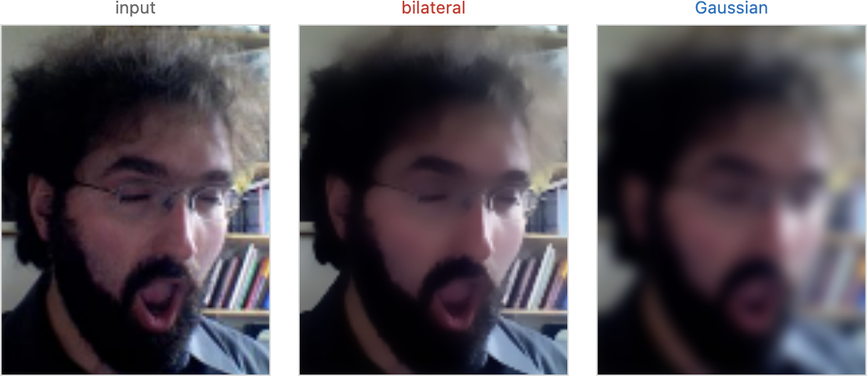
The 1-D picture carries straight to the 2-D image: the bilateral smooths flat texture and noise inside each region while holding the edges, so a portrait emerges with clean skin and intact eyelashes, and an HDR base layer stops cleanly at the silhouette instead of ramping across it (Figure 5.2.3).

One observation lifts the bilateral from a useful trick to the organizing idea of the whole chapter. The range Gaussian $g_r$ is not just a clever weight — it is a similarity, an affinity between two pixels: a number that says how much these two pixels belong together, computed from their value difference. The bilateral averages pixels in proportion to that affinity. Every later method in this chapter — and several beyond it — is a different answer to one question: how should we measure whether two pixels belong together?
Use the color / intensity difference between two pixels as how much they belong together — an affinity — then average (or connect) pixels in proportion to it. Pixels with high affinity are treated as measurements of the same underlying thing and get averaged together; pixels with low affinity — across an edge — are kept apart. The bilateral filter's range weight $g_r$ is the first full instance, but the same affinity drives the bilateral grid, the guided filter, non-local means (NL-means), colorization, and matting / segmentation that follow. Edge-preserving is affinity. (This is L4, registered in Denoising where the bilateral first appeared for noise; this is its full edge-preserving treatment.)
Robustness for values with few neighbours⧉
The normalized form above carries a quiet weakness, and it bites exactly where it should not. Consider a pixel whose value is rare — a lone bright speck against a dark wall, a thin highlight, a pixel sitting on a tiny isolated feature. Very few of its neighbours fall within $\sigma_r$ of its value, so its normalizer $W_p = \sum_q w(p,q)$ is tiny and noisy: a sum of a mere handful of small weights. Dividing by a near-zero $W_p$ amplifies whatever noise those few neighbours carry, and the standard normalized average over-trusts them. In this regime the Durand–Dorsey normalization is, strictly, the wrong thing to do — it manufactures a confident estimate out of almost no evidence.
The fix is to stop dividing, and to express the output as a correction to the input rather than a fresh average built from scratch (Aubry et al. 2014). Write the bilateral output as the input plus a sum of per-neighbour pulls, and drop the $1/W_p$:
This is the unnormalized, or delta, bilateral. Read each term: a neighbour $q$ contributes $w(p,q)\,(I_q - I_p)$, a nudge toward its own value scaled by how much it belongs. When many neighbours match — a flat region — these nudges accumulate and pull the pixel firmly toward the local consensus, just as the normalized filter does. But when few neighbours match — a rare value — the nudges are few and small, so the pixel makes a small correction and stays close to itself, instead of dividing by a near-zero $W_p$ and blowing up. A lonely value is left roughly alone, which is the honest answer when there is little to average it against.
This unnormalized form is also the bilateral cousin of the local Laplacian filters: working in deltas from the input, scale by scale, is exactly the move that makes the multiscale local Laplacian fast and robust (Paris / Aubry; cross-ref Local Laplacian filters and Linear pyramids and wavelets).
The delta form above is more than a normalization fix: it is one step of gradient descent on a robust energy, and that observation ties the bilateral filter to a second classic family — anisotropic diffusion. Read $\sum_q w(p,q)\,(I_q-I_p)$ as a weighted, edge-stopping diffusion of intensity: where neighbours agree (small $|I_q-I_p|$) heat flows freely and the region smooths; where they disagree across an edge (large $|I_q-I_p|$) the weight $w$ collapses and flow stops. That is exactly Perona–Malik anisotropic diffusion (Perona & Malik 1990) — iterate $\partial_t I = \operatorname{div}\!\big(g(|\nabla I|)\,\nabla I\big)$ with a conductance $g$ that vanishes for large gradients, and edges survive because no heat crosses them. The bilateral filter is essentially a large-step, non-iterated version of the same idea. What unifies them is robust statistics (Black et al. 1998; Durand & Dorsey 2002). Smoothing a pixel toward its neighbours is estimation: minimize a penalty $\sum_q \rho(I_q-I_p)$ on the value differences. A quadratic penalty $\rho(x)=x^2$ lets every neighbour pull in proportion to its difference — so large differences (edges) pull hardest, and the estimate is the plain average that blurs edges. Swap in a robust penalty that saturates (Lorentzian, Tukey biweight) and its derivative — the influence function $\psi=\rho'$ — rises and then returns to zero for large differences: a neighbour across an edge is an outlier and exerts no pull. Perona–Malik's conductance $g$, the bilateral's range weight $g_r$, and a robust influence function are the same curve — edge preservation is just outlier rejection (Figure 5.2.5). The idea generalizes from a scalar conductance to a tensor one — diffusion that flows along a structure but not across it. That is the basis of diffusion-tensor imaging (DTI) in medicine: each voxel carries a $3\times3$ diffusion tensor (drawn as an ellipsoid, elongated along the direction water moves most freely), estimated from the diffusion of water in tissue, which lets tractography trace white-matter fibre bundles in the brain (Figure 5.2.6).


Debugging — hand-checkable limits⧉
The bilateral has two limits you can predict by hand, and together they make an excellent correctness test for an implementation (Figure 5.2.7). Push the range width to each extreme:
- Large range variance ($\sigma_r \to \infty$): the range Gaussian flattens, $g_r \to 1$, so it does nothing — every value difference counts as "similar." The weight reduces to the spatial Gaussian alone, and the bilateral collapses to a plain Gaussian blur.
- Tiny range variance ($\sigma_r \to 0$): only neighbours with essentially the identical value survive, which in practice means the pixel itself. The filter refuses to average anything, and the output is the identity — the image comes back untouched, edges and all.
A middle $\sigma_r$ interpolates between these two: enough to smooth away noise and texture, not so much that it bleeds across real edges. If your implementation does not reproduce a Gaussian at large $\sigma_r$ and the identity at small $\sigma_r$, it is wrong — these are the first two things to check (and the recipe in the debugging sidebar above).

The same two knobs guide tuning. Pick $\sigma_s$ from the spatial scale of the structure you mean to remove (how large a region should be pooled). Pick $\sigma_r$ from the contrast of the edges you mean to preserve — set it just below the value jump of a real edge, so the filter smooths everything gentler than that and stops at anything sharper. And state the encoding first: the same numeric $\sigma_r$ means something completely different in linear light, in gamma, and in log luminance.
5.2.3 Cross / joint bilateral⧉
So far the affinity has been read off the same image we are smoothing — the range weight uses $I$ itself. But there is no reason it must. The cross (or joint) bilateral filter reads the range weight from a different image, a guide $J$, while still averaging the target $I$:
The averaging runs over the target $I$; the affinity comes from the guide $J$. Why want that? Because sometimes the image you wish to smooth is too noisy or too dark for its own edges to be trusted — read the affinity off $I$ and you are reading off the noise. If you hold a cleaner signal that shares the same scene geometry, borrow its edges instead.
The headline application is flash / no-flash photography (Petschnigg et al. 2004; Eisemann & Durand 2004). Shoot a dim scene twice: once without flash (the right mood and color, but dark and noisy) and once with flash (clean and well-exposed, but flat, harsh lighting). The two share the same edges — the same object boundaries are present in both. So smooth the noisy no-flash image using the flash image as the guide: the flash image's clean edges drive the range weight, telling the filter where it may and may not average, while the values being averaged come from the ambient no-flash shot. The result keeps the no-flash mood and kills the no-flash noise (Figure 5.2.8). We develop the full flash/no-flash pipeline later (forward-ref → #Illumination related effects in a single image, computational illumination).

The cross bilateral is the first instance of a more general joint / guided idea — filter one image using structure taken from another — that culminates in the guided filter (later in the part).
5.2.4 Bilateral grid⧉
The bilateral filter is non-linear: the weights depend on the pixel values, so they differ at every output pixel, and the whole thing is not a convolution. That is why you cannot reuse your fast Gaussian-blur code, and why a brute-force bilateral is a slow double loop. The bilateral grid (Chen, Paris & Durand 2007) is the beautiful observation that you can turn it back into an ordinary convolution — by adding a dimension (Figure 5.2.9).
The key picture: the product of a spatial Gaussian (in $x, y$) and a range Gaussian (in $I$) is just a single 3-D Gaussian in the space $(x, y, I)$. So lift every pixel out of the 2-D plane into a 3-D space by using its value as a third coordinate — pixel $(x, y)$ with value $I(x, y)$ goes to grid position $(x, y, I(x,y))$. In this lifted space the nonlinear 2-D bilateral becomes a plain, separable 3-D Gaussian blur — an ordinary linear convolution — and the edge-preserving behaviour is now automatic: two pixels on opposite sides of an edge have very different values, so they land in different layers of the grid, and a 3-D blur simply cannot reach between them.
The pipeline has three steps — splat, blur, slice:
- Splat. Build a coarse 3-D grid indexed by $(x, y, I)$. For each pixel, accumulate two things into its cell: its value and a weight (a count of how many pixels landed there). Many cells receive no pixels and stay empty; the per-cell weight is exactly the bookkeeping that will reproduce the bilateral's normalizer.
- Blur. Convolve the grid with a plain separable 3-D Gaussian — an ordinary blur along each axis in turn (the $[1\ 4\ 6\ 4\ 1]/16$ stencil if the Gaussian is one cell wide). Blur both the accumulated values and the weights. Spatial smoothing and range smoothing both fall out of this single convolution; dissimilar values never mix because they live in different $I$-layers.
- Slice. Read the result back out at each pixel's own location $(x, y, I(x,y))$ by trilinear interpolation, and divide the interpolated value by the interpolated weight — that division is the bilateral normalizer $1/W_p$, recovered for free.
The whole pipeline is short, and every step is an ordinary operation — accumulate, blur, look up:
# splat — build the coarse grid (downsample by σ_s in space, σ_r in range)
for each pixel (x, y):
    c ← (x/σ_s, y/σ_s, I[x,y]/σ_r)      # the cell this pixel lands in
    grid[c]   ← grid[c]   + I[x, y]      # accumulate value
    weight[c] ← weight[c] + 1            # accumulate count

# blur — plain separable 3-D Gaussian, on BOTH grid and weight
blur grid, weight along x, then y, then I    # e.g. [1 4 6 4 1]/16 per axis

# slice — read back at each pixel's own (x, y, I), normalized
for each pixel (x, y):
    c ← (x/σ_s, y/σ_s, I[x,y]/σ_r)
    out[x, y] ← grid[c] / weight[c]      # trilinear interpolation at c
return out
Why is this fast? Because the grid is coarse. The right resolution is set by the filter's own widths — a grid cell about $\sigma_s$ wide in space and $\sigma_r$ deep in range — so the grid is heavily downsampled in both space and value, often by large factors. A small grid, a separable blur, a trilinear read: the whole thing runs in real time on a GPU. This is the pipeline that Halide schedules for live bilateral filtering (cross-ref #Differentiable image pipelines and algorithm optimization (Halide)).

The grid also makes the affinity lesson geometric: the third axis is the affinity, drawn as a coordinate. Two pixels far apart in value are literally far apart in the grid, so a local blur — which only mixes nearby cells — can never average them together. The bilateral's "do these pixels belong together?" becomes, in the grid, simply "are these cells close?"
5.2.5 Bilateral-grid learning (HDRnet)⧉
The grid stores, per cell, a value and a weight — a small, edge-aware, low-resolution summary of the image from which a full-resolution result is sliced. HDRnet (Gharbi et al. 2017, Deep Bilateral Learning) takes the obvious next step: rather than fill the grid by splatting the input, learn what goes in it. A convolutional neural network runs on a low-resolution copy of the image and predicts, per grid cell, the coefficients of a per-cell affine transform — a little color/tone map to apply. Then, at full resolution, the network slices that grid at each pixel's $(x, y, I)$ (an edge-aware, trilinear lookup) and applies the sliced affine transform to the original pixel.
This is best-of-both once more: run a heavy network on a tiny image (cheap, and able to capture a global, learned enhancement), then carry the result back to the full-resolution image through an edge-aware upsampling structure that keeps the detail crisp. The bilateral grid has become a learned, edge-preserving upsampling layer — fast enough to run live on a phone. It is also a clean instance of swapping a hand-designed operator for a learned one (a one-line callback to L8; cross-ref Machine learning).
Big lessons of this chapter
The recurring principles from this chapter, gathered for review.
Use the color / intensity difference between two pixels as how much they belong together — an affinity — then average (or connect) pixels in proportion to it. Pixels with high affinity are treated as measurements of the same underlying thing and get averaged together; pixels with low affinity — across an edge — are kept apart. The bilateral filter's range weight $g_r$ is the first full instance, but the same affinity drives the bilateral grid, the guided filter, non-local means (NL-means), colorization, and matting / segmentation that follow. Edge-preserving is affinity. (This is L4, registered in Denoising where the bilateral first appeared for noise; this is its full edge-preserving treatment.)