2.10 Photography and camera 101🔗⧉

We have built the physics of image formation: rays selected by a lens, projected by perspective, integrated over the aperture and the pixel and the exposure time, and counted as photons on a sensor. Now we sit behind a real camera and ask the practical questions. Which dial does what, and what does it cost? How does the camera decide the exposure on its own, and when does it get it wrong? How does autofocus find the focus plane, and how does a phone — with a sensor the size of a fingernail and no aperture ring at all — produce a picture that rivals a camera ten times its size? This chapter is the bridge from the abstractions of the previous chapters to the buttons under your thumb, and from there to the computational chapters that make a phone camera work.

The throughline is that every control on a camera is one of the previous chapters made physical. The aperture ring sets the $f/D$ ratio from the lens chapter; the shutter dial sets the exposure time $t$ from the sensor integral; the ISO setting scales the gain that the noise section described; the focus ring moves the image distance $v$ of the thin-lens equation. Learn the physics once and the camera stops being a box of mysterious modes.

2.10.1 Basic photography: exposure settings — shutter, aperture, and ISO🔗⧉

How bright a photo comes out is its exposure, and from the radiometry and sensor chapters we already have the equation: exposure is irradiance times time, and the irradiance the lens delivers scales with aperture area, so

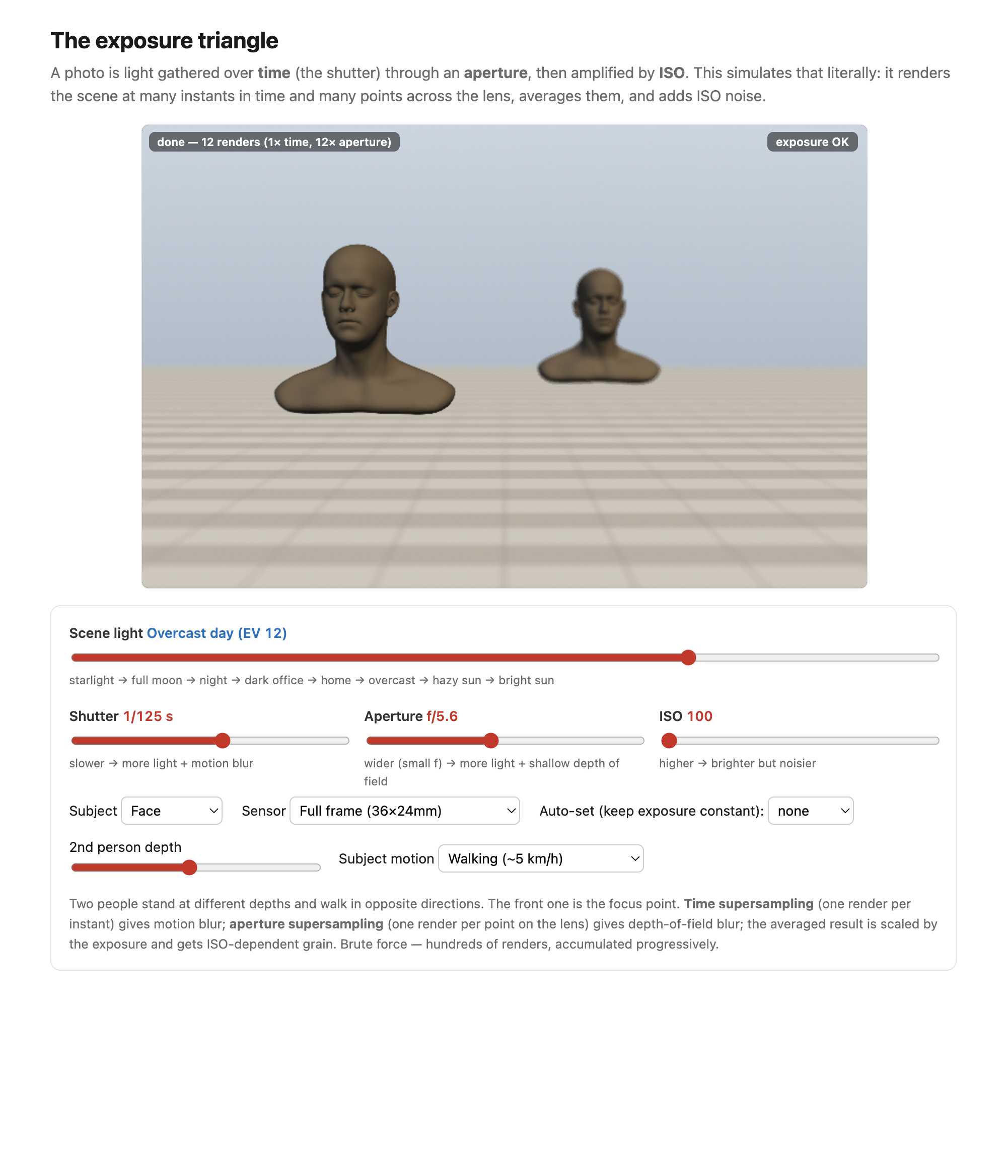
Two optical controls set it. Shutter time $t$ enters linearly — twice the time, twice the light. Aperture enters through its area, which goes as the diameter squared $D^2$, i.e. as $1/N^2$ in the f-number $N = f/D$ — so twice the f-number means a quarter the light. This is finally why photographers describe the aperture by the ratio $f/D$ rather than the raw diameter: a longer lens at the same f-number has a proportionally bigger opening, so it gathers the same light per unit of sensor area despite seeing a narrower field of view. The longer lens divides the world into a smaller patch (less light per pixel from the geometry) but compensates with a larger physical aperture (more light gathered), and the ratio $f/D$ is exactly the quantity that nets those two effects out. The ratio normalizes light-gathering across focal lengths — precisely what you want a brightness setting to do.

A third control, ISO, is electronic rather than optical: it scales the gain applied to the sensor signal after capture. Raising ISO does not collect more light; it amplifies what was collected, brightening a dim exposure at the cost of also amplifying noise (the sensor chapter's read and shot noise). So the three legs of exposure are shutter, aperture, and ISO — two that change the light and one that changes the gain.

Each control carries a side effect you cannot escape, and each was derived elsewhere in this part. A longer shutter time risks motion blur of anything that moves during the exposure (covered fully in Motion/Video); a wider aperture (smaller $N$) shrinks the depth of field (DoF) — the range of distances in acceptable focus (the lens chapter); and a higher ISO raises noise (the sensor chapter). Choosing an exposure is therefore never a single decision but a negotiation among brightness, motion, depth of field, and noise (Figures 2 and 3).

Stops and the power of two. Photographers do not count light in raw multiples; they count it in stops, where one stop is a factor of two in light — the natural unit because the eye and the medium respond to ratios, not differences (the same logarithmic perception behind gamma encoding, in Color technology). One stop brighter is $+1$ exposure value (EV), so a stop is a log₂ unit: $\text{stops} = \log_2(\text{light ratio})$, with $\mathrm{EV} = \log_2(N^2/t)$. This is why the classic f-number series looks so irregular — $f/1.4, f/2, f/2.8, f/4, f/5.6, f/8, f/11, f/16$. Because light $\propto$ aperture area $\propto D^2 \propto 1/N^2$, each step multiplies $N$ by $\sqrt{2}$, so the area — and the light — halves at every step (Figure 2.10.3). Shutter speeds ($1/30, 1/60, 1/125, \dots$ s) and ISO ($100, 200, 400, \dots$) step in the same power-of-two stops; cameras add ⅓-stop clicks for fine control. The point is that one stop of aperture, one stop of shutter, and one stop of ISO all change the brightness by the same factor — they are interchangeable currency, the exposure triangle (Figure 2.10.5).

Autoexposure and metering. How does the camera pick an exposure on its own? Its meter integrates the scene's light — through the lens (TTL — through-the-lens), as a center-weighted average, a narrow spot, or a smart evaluative/matrix reading — and then renders that average to a mid-gray assumption: it assumes the average scene reflects about 18% gray and sets the exposure to make it so. This works for ordinary scenes and fails predictably on high- and low-key ones (Figure 2.10.6). A snowfield is far brighter than 18% gray, so the meter, dragging it down to gray, underexposes — the snow comes out dingy, and you must dial in $+1$ or $+2$ EV to put it back. A black cat fills the frame with something far darker than gray, so the meter overexposes it to muddy gray, and you dial in $-$EV. Smart matrix metering — Nikon's 3D Color Matrix, learned from a database of tens of thousands of photographs — adds brightness, color, contrast, and distance cues to guess the photographer's intent, but metering remains, in essence, an open problem.

Priority modes. Because shutter and aperture trade off, cameras offer priority modes: in aperture priority you set $N$ (and thus depth of field) and the camera picks the shutter $t$; in shutter priority you set $t$ (and thus motion blur) and the camera picks $N$. Aperture priority is the usual default, because depth of field is usually the creative variable. Each mode fails when no valid partner exists: ask for $f/1.4$ in blazing sun and the required shutter may be faster than the camera can go; ask for $1/1000$ s in a dim room and no aperture is wide enough. (The full mode dial gets its own section next.)

Expose to the right. A subtle but important habit, which the noise section justifies: expose to the right (ETTR) — push the exposure as bright as you can without clipping the highlights, so the histogram piles up toward the right edge (Figure 2.10.7). The reason is that noise lives in the shadows (the signal-to-noise ratio is worst where photons are fewest), so capturing more light everywhere, especially in the darks, improves quality; you pull the brightness back down later in software at no cost. And when you do need to brighten, raising the ISO in-camera beats brightening in software, because ISO gain amplifies the signal together with the early (pre-amplifier) noise but not the later read noise added on readout — so the signal gets a head start over part of the noise. ETTR and ISO are both the noise section's logic applied at capture time.

2.10.2 Exposure modes, UI, and auto-ISO🔗⧉

The mode dial looks like a menagerie, but underneath it is just who picks which leg of the exposure triangle. The four classic program, aperture-priority, shutter-priority, and manual (PASM) modes are exactly the four answers (Figure 2.10.8):

• P (program) — the camera picks both aperture and shutter from the meter, and you can "program-shift" to slide along the equally-exposed pairs (more aperture, faster shutter, and vice versa).
• A / Av (aperture priority) — you set the aperture (and thus the depth of field), the camera picks the shutter.
• S / Tv (shutter priority) — you set the shutter (and thus the motion rendering), the camera picks the aperture.
• M (manual) — you set both, and the meter only advises.

Beyond these sit full Auto and the scene modes (portrait, sports, night), which are presets that bias the program toward a guessed intent.

Auto-ISO is the modern fourth knob, and it changes the logic. In plain A or S the camera still has only one free leg, so a single setting can over- or under-expose when the light is extreme. Auto-ISO frees a second leg by letting ISO float: now you can hold both a chosen aperture and a minimum shutter speed, and let the ISO climb to make the exposure work. You cap the maximum ISO (your noise budget) and a minimum shutter speed — often a "1/focal-length" rule (so a 200 mm lens won't drop below 1/200 s) or a multiple of it. This is why M + auto-ISO has become a popular combo: you nail aperture and shutter for the look you want, and let ISO be the automatic variable, with exposure compensation still steering it.

Exposure compensation (±EV) is the manual override for the meter's 18%-gray failure without leaving an auto mode: it biases the mid-gray target, so a snow scene gets $+$EV and a dark scene $-$EV. On a mirrorless body the dedicated dial and the live exposure meter make this immediate — you see the brightness change before you press the shutter, the subject of the UI and display section below.

2.10.3 Focus, autofocus, and depth of field🔗⧉

Focusing, from the thin-lens chapter, is nothing more than choosing the image distance $v$ — moving the lens so the subject's image lands exactly on the sensor. Doing that automatically, fast and accurately, is autofocus (AF), and there are two classic passive families plus a modern on-sensor synthesis (Figure 2.10.9).

Contrast-detection autofocus (CDAF) drives the lens until the image contrast (sharpness) is maximal. It is accurate — the peak of the sharpness curve is exactly best focus — but it has to hunt: from a single blurred frame it knows only that the image is soft, not which direction sharpens it, so it must dither past the peak to find it. Historically slow, it was the staple of early mirrorless bodies and compacts.

Phase-detection autofocus (PDAF) is cleverer. It looks at the scene through two opposite edges of the lens — two sub-apertures — giving two slightly shifted views of the same scene. The phase difference between them gives the direction and the amount of defocus in a single shot, so the lens drives straight to focus with no hunting (Figure 2.10.10). This is literally a tiny stereo measurement (the two sub-apertures are a micro baseline), and it is why the next chapter's stereo geometry shows up inside a single camera. The classic single-lens reflex (SLR) implemented PDAF with a dedicated AF sensor hidden under the reflex mirror.

On-sensor PDAF and dual-pixel is the modern synthesis that mirrorless bodies use. Instead of a separate AF sensor, phase detection is moved onto the imaging sensor itself — either with scattered masked AF pixels, or with dual-pixel designs that split every photosite into two halves that see opposite sub-apertures. The result is phase detection at nearly every pixel, the speed of PDAF with the coverage of CDAF — the best of both worlds. (Those same split photosites are a literal micro-stereo pair, which is how Google's Pixel computes the depth for its portrait-mode background blur.) For completeness, active AF — old Polaroid sonar (ultrasonic time-of-flight) and infrared rangefinding — works in the dark but is crude; it is distinct from an AF-assist lamp, which merely throws contrast onto the subject so passive AF can work.

Depth-from-defocus AF (Panasonic DFD) is a third route that wrings a one-step focus cue out of an ordinary contrast sensor — no phase pixels at all. The trick is to model how a particular lens blurs: knowing its point-spread function as a function of focus, the camera shoots two frames at slightly different focus and reads off, from how the blur changes between them, both the direction and the amount of defocus. That is a PDAF-like single-step estimate sitting on top of a plain contrast sensor — it still rides on CDAF for the final confirmation, and it needs a per-lens blur profile baked in (so it works only with the maker's own lenses). The full treatment of how defocus encodes depth is deferred to the Optics part (Focus).

Focus modes decide whether to lock or track: AF-S / one-shot locks focus once, for still subjects; AF-C / AI-Servo tracks continuously and even predicts motion, for action. Increasingly, what to focus on is itself automated: from single-point and zone selection, cameras have moved to subject-detection AF that finds and tracks a face → eye → animal / bird / vehicle with a deep-learning detector (→ Machine learning). Eye-AF is the headline modern feature for portraits — the camera locks the nearest eye and holds it as the subject moves. Two handling tricks round out the section: back-button focus decouples AF from the shutter button (focus with a thumb button, release with the shutter), and focus-and-recompose locks focus on the subject, then reframes — but beware the small focus-plane error this introduces at wide apertures and close range, where depth of field is razor-thin.

2.10.4 Lenses and focal length🔗⧉

Focal length sets the field of view — the geometry was derived in the Pinhole chapter, including the "35 mm" / crop-factor sidebar — so here we treat lenses as a photographer chooses them: what each focal length is for, and what fast/slow and prime/zoom buy you.

Primes versus zooms. A prime lens is one fixed focal length; for the same quality it is typically brighter (faster), sharper, smaller, and cheaper, and it "makes you think and move your feet." A zoom trades some of that for the convenience of many framings in one lens. A cheap fast prime — a 35 mm or 50 mm or 85 mm at f/1.8 — is some of the best value in photography: razor-sharp and bright for the price. Modern zooms are excellent, but the basic kit zoom is usually a camera's weakest optical link.

The focal-length families (quoted on full frame; remember the crop factor for smaller sensors), each with what it is for (Figure 2.10.13):

• ultrawide (≤24 mm): landscapes, interiors, exaggerated near/far — but watch the perspective stretch at the edges.
• wide (~24–35 mm): environmental and reportage work — "the subject and its context."
• normal (~50 mm): close to the eye's own perspective, unobtrusive, and usually fast and cheap.
• short telephoto (~85–135 mm): portraits — the working distance gives flattering proportions and easy subject separation (and the reason is distance, not the lens — see below).
• telephoto / super-telephoto (~200 mm and up): sports, wildlife, the moon — strong compression, bringing far subjects close.

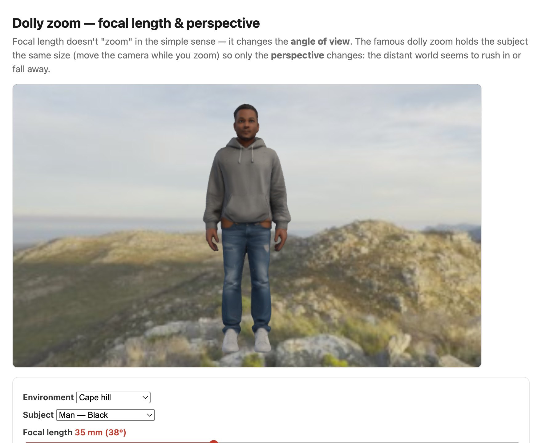
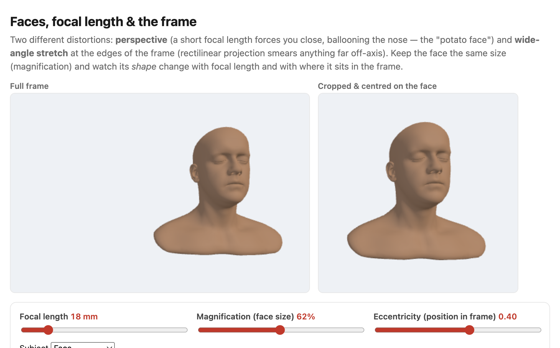
Why portrait lenses flatter — it is the distance, not the lens. It is tempting to credit the "portrait" focal length itself for flattering a face, but the lens is only an accomplice. What actually shapes a face is the camera-to-subject distance, and the same focal-length-versus-distance distinction the Pinhole chapter drew for backgrounds governs faces too. Up close — where a wide lens forces you to stand to fill the frame — the nose is markedly nearer the lens than the ears, so by the perspective $1/Z$ falloff it looms: a bulbous nose, an inflated forehead, ears that recede into nothing. Step back and shoot from a few meters with a short telephoto and those front-to-back distances equalize, so the proportions read as natural. The "portrait" focal length (~85–135 mm) flatters precisely because, at a normal framing, it makes you back away to that comfortable distance; the longer focal length is just what crops the now-distant face back to a head-and-shoulders. The striking finding is that the chosen distance changes not only proportions but perceived personality: in rating studies, faces shot from closer are judged less trustworthy, less competent, and less attractive — a sub-meter change in where you stand measurably shifts how a stranger is read (Perona 2007; Bryan et al.). The flip side — the gross wide-angle face stretch when you cannot back away, as on a phone's selfie camera, and how to undo it computationally — is the subject of Perspective distortion and its correction.

Fast versus slow. A fast lens has a large maximum aperture (small f-number, e.g. f/1.4) — more light and shallower depth of field; a slow lens (f/5.6) is smaller and cheaper but light-starved. Zooms are often slow, and many have a variable maximum aperture that shrinks as you zoom in (e.g. f/3.5 wide, f/5.6 long). The "35 mm-equivalent" reminder is worth repeating but not re-deriving: a focal length only means a field of view relative to a sensor size, so smaller sensors crop and you multiply by the crop factor (APS-C ≈ 1.5×, Micro Four Thirds ≈ 2×, phones much more) to compare — see the Pinhole chapter's "35 mm" sidebar.

2.10.5 Lens filters: polarizers, ND, and graduated ND🔗⧉

A few pieces of glass screwed onto the front of the lens change which light the sensor captures — and the most interesting of them do something software cannot redo afterward (Figure 2.10.14).

The circular polarizer (CPL). Natural light is unpolarized (its electric field oscillates in a rapidly varying mix of directions), but reflection off a non-metal surface — water, glass, wet leaves — partially polarizes what bounces off it, and so does the blue sky (skylight is most strongly polarized in a band about $90°$ from the sun). A polarizer is a rotatable filter that passes only one polarization, so turning it lets you cut glare and reflections off those surfaces, deepen a blue sky, and boost saturation as the haze of scattered, polarized light is removed (this is the polarization of the Reflection sidebar, put to work). It costs about 1–2 stops of light, and it is "circular" — a linear polarizer followed by a quarter-wave plate — specifically so that the camera's beam-splitter-based autofocus and metering still see unpolarized light and keep working. Crucially, its effect is not reproducible in post: it changes the light before capture, so no slider can recover the un-glared, deep-sky image from a shot taken without it.

Neutral-density (ND) filters. An ND is a uniform gray that cuts the light by a chosen number of stops with (ideally) no color shift — a brightness knob in glass. Its point is to let you choose a setting you otherwise could not in bright light: a slow shutter for silky water or motion blur, or a wide aperture for shallow depth of field under a midday sun. Strong NDs (6–10 stops) make daytime long exposures possible; a variable ND is simply two stacked polarizers, rotated against each other to dial the strength continuously.

Graduated ND (GND). A graduated ND is dark at the top and clear at the bottom, with a hard, soft, or reverse transition. Lined up with the horizon, it holds back a bright sky so a high-contrast landscape fits inside a single exposure — an optical alternative to HDR bracketing (→ Image measurements; Multiple exposure), done in glass at capture time rather than by merging frames later.

UV / protective filters. A clear or UV filter today is mostly lens protection (it once cut UV haze on film); whether the protection is worth adding one more glass surface that can introduce flare is a perennial photographers' debate.

The throughline ties the section back to the chapter's bigger argument: the polarizer's and GND's effects are largely un-doable in software — the polarizer changes the captured light itself, and the GND is a per-shot exposure blend — which is exactly why these physical filters survive into the computational era, whereas a plain ND (which only scales brightness, something software can fake) is the one whose job a computer can take over.

2.10.6 Keeping the lens clean🔗⧉

A smudged or dusty front element is not a cosmetic problem — it is an optical one. Stray light hitting the dirt scatters across the frame, producing veiling flare, lowering contrast, and casting soft dust spots (worst when stopped down, where the spots come into focus). Clean glass is real image quality, not fussiness.

There is an order of operations, gentlest first, because each step risks the delicate anti-reflection coating. Start with a blower to lift loose grit without dragging it across the glass; then a soft brush; then a microfibre cloth or lens pen; and only for stubborn smears, a drop of lens fluid. Wipe gently and from the centre outward, and never dry-wipe a gritty element — that grinds the grit into the coating.

The companion warning is don't overdo it: every wipe is a small risk to the coating, and a little dust is optically harmless (it is far out of focus and scatters a negligible fraction of the light). A protective / UV filter or simply the lens hood prevents most of the problem in the first place. The cousin problem is sensor dust — but those spots sit in a fixed place in the frame (they do not move when you change lenses or zoom), which is the giveaway. Cameras fight it with an in-body ultrasonic shake of the sensor at startup; beyond that, a rocket blower or a wet swab cleans it, and dust-mapping lets software paint the spots out automatically (→ dust-spot removal, BASIC).

2.10.7 Image stabilization🔗⧉

A long exposure handheld blurs not only moving subjects but the whole frame, from the tiny tremor of your hands. Image stabilization fights that camera shake: a gyroscope senses the camera's angular shake and a feedback loop counters it during the exposure, letting you hand-hold slower shutter speeds — typically a gain of 2–5 stops (so a shot that needed 1/100 s can succeed at 1/4 s). There are three implementations (Figure 2.10.15):

• Optical image stabilization (OIS) — in-lens: a floating lens element shifts to counter the shake (Canon's image stabilization (IS), Nikon's vibration reduction (VR)). Tuned per lens, it also steadies the viewfinder and the AF system.
• In-body image stabilization (IBIS) — the sensor itself rides a moving stage and counter-shifts. It works with any mounted lens, can stack with OIS, and the same moving stage enables sensor-shift high-resolution modes.
• Electronic / digital image stabilization (EIS) — crop a margin and warp each frame to cancel the motion. Cheap, with no moving parts (phones and video use it), but it costs resolution and field of view and can add a "wobble" artifact.

The crucial limit: stabilization fixes camera shake, not subject motion. A stabilized 1/4 s shot of a static scene is sharp, but a moving subject in that same frame still blurs — for that you need a fast shutter. This is a common beginner confusion, worth stating flatly: stabilization buys you slow shutters for still subjects only.

2.10.8 UI and display🔗⧉

A camera's controls are abstractions; its viewfinder and display are where those abstractions become visible feedback — and this is exactly what mirrorless changed (Figure 2.10.16).

Viewfinders. An optical viewfinder (OVF) — the SLR's mirror-and-prism, or a rangefinder's window — shows the real world directly: zero lag, infinite resolution, but it does not show the captured exposure or white balance, only the scene. An electronic viewfinder (EVF) (and the rear LCD) shows the sensor's live feed instead: slightly laggy, but what-you-see-is-what-you-get. Exposure, white balance, and even a depth-of-field preview are all visible before you press the shutter.

Exposure preview and the live histogram. Because the EVF or LCD can simulate the captured image, it can overlay a live histogram to judge clipping in real time — which is the practical home of ETTR: push the histogram to the right without letting the highlights pile up against the right edge.

Focus aids. For manual focus, focus peaking highlights the high-contrast (in-focus) edges, and a magnify mode zooms in to check critical focus. For exposure, zebras — animated diagonal stripes over near-clipped highlights, borrowed from video — warn you before you blow out the brights.

The throughline: an EVF turns the abstractions of exposure and focus into direct visual feedback, which is why mirrorless changed how people shoot — you stop guessing and start seeing the photograph before you take it.

2.10.9 Video modes🔗⧉

Video is a stack of exposures, so most of it forward-references the dedicated Motion/Video chapter; here we name just the controls a stills photographer meets when they hit the record button.

• Frame rate and shutter angle. Video sets the exposure time as a fraction of the frame interval. The 180° shutter-angle convention — shutter open for about half the frame time — gives the "natural" amount of motion blur that reads as cinematic; too short a shutter looks stuttery, too long looks smeared. A high frame rate (shot then played back slower) gives slow motion.
• Rolling shutter and "jello." A complementary metal-oxide-semiconductor (CMOS) sensor reads out row by row (the sensor chapter), so during fast motion — a quick pan, a spinning propeller — the top and bottom of the frame are captured at slightly different instants and the image skews or wobbles, the "jello" effect. A global shutter (every pixel exposed at once) avoids it but is rarer and costlier.
• Log profiles and grading. Shooting a log (flat, low-contrast) profile preserves dynamic range across the frame, to be color-graded in post — the video cousin of shooting raw and applying a tone curve later.
• Codecs and bitrate. Intra- versus inter-frame compression, 8- versus 10-bit, chroma subsampling (4:2:0 vs 4:2:2), and bitrate all trade file size against editing and grading headroom.

The algorithms behind all of this — and the full treatment of motion — live in the Motion/Video chapter; this section is deliberately brief.

2.10.10 Programmability, or the lack thereof🔗⧉

Here is an obstacle that shapes this entire book. Most cameras run closed firmware: you cannot run your own code on them. The computational-photography ideas in the chapters ahead — multi-frame high-dynamic-range merging, burst denoising, computational bokeh — all need programmable capture: control of the per-frame exposure, focus, and gain, and access to the raw burst before the camera's own pipeline mangles it. A stock camera grants none of this, so its computational ideas cannot even be tried on most cameras (Figure 2.10.17).

The community responded with hacks: CHDK (Canon Hack Development Kit, for PowerShot compacts; CHDK (Canon Hack Development Kit)) and Magic Lantern (for Canon DSLRs; Magic Lantern) are add-on firmware that expose scripting, raw video, auto-bracketing, intervalometers, and focus stacking — features born precisely because the manufacturers withheld them. The open road, though, runs through phones: Android's Camera2 / CameraX API (and Google's earlier FCam research camera) expose per-frame control of exposure, focus, and gain, plus access to the raw burst. That openness is why phones, not cameras, became the home of computational photography — the platform that grants programmable capture is the platform where the research happens, and it is the bridge to the rest of this book.

There is also a maker road, the most open of all: a Raspberry Pi with a camera module (the HQ camera, driven by the libcamera / picamera2 stack) is a cheap, fully open, fully programmable camera. It hands you per-frame control of exposure and gain and direct access to the raw Bayer frames on a hobbyist board you can script in a few lines of Python — which makes it the natural platform on which to try this book's algorithms and build a do-it-yourself computational camera.

2.10.11 Anatomy of a modern full-frame interchangeable-lens camera🔗⧉

It helps to see the whole machine at once, because each block is a previous section made physical (Figure 2.10.18). Trace the light from front to back through a modern mirrorless body:

Lens and mount (electronic contacts carry autofocus, aperture, and stabilization signals) → sensor on an IBIS stage (the moving sensor of the stabilization section) → shutter — a mechanical curtain and/or an electronic rolling shutter (the readout of the sensor chapter) → image processor and AF — on-sensor PDAF, subject detection, and the image signal processor (ISP, the computational pipeline of the next part) → EVF and rear LCD (the live feed of the UI section) → card and battery.

The defining change from the single-lens reflex (SLR) is that the mirror box and optical prism are gone. In an SLR, a 45° mirror bounced the lens's image up into an optical prism and the OVF, then flipped up out of the way at the instant of exposure. Remove it, and the sensor feeds the EVF directly — which is exactly what enables WYSIWYG preview, on-sensor PDAF spread across the whole frame, a silent electronic shutter, and a shorter lens-to-sensor (flange) distance that allowed the new, smaller lens mounts. The mirrorless body is the SLR with its one big moving part removed and the sensor promoted to do the viewfinder's job.

2.10.12 Anatomy of cell-phone cameras🔗⧉

A phone reaches the same goal — a good photograph — by a wholly different route, and the difference is the punchline of the chapter (Figure 2.10.19). Its hardware is constrained: a tiny sensor behind a bright, fixed-aperture lens. There is no iris, so exposure is set by shutter and ISO alone. The tiny sensor has two consequences that fall straight out of earlier chapters: depth of field grows as the sensor shrinks (the lens chapter), so a phone has enormous depth of field and must fake background blur; and a small sensor collects fewer photons, so it has more noise and must burst-and-average to clean it up.

Where a camera uses a zoom lens, a phone uses a multi-camera array: separate ultrawide / wide / tele modules, the long end often a periscope that folds the light path sideways with a prism so a long focal length fits a thin body. "Zooming" really means switching cameras (with cropping and fusion in between).

The key idea is that the computational pipeline does the heavy lifting that the optics cannot: demosaicking, multi-frame high dynamic range (HDR; the HDR+ pipeline) and burst denoising, computational bokeh (depth from the dual-pixel split or the multi-camera array), night mode, and super-resolution. The phone overcomes small-sensor physics with computation rather than glass — forward-referencing the Basic ISP and Multiple-exposure parts, where these algorithms live. This is the chapter's punchline and the book's bridge: cheap optics plus a smart pipeline beats good optics alone.

2.10.13 Types of cameras🔗⧉

The two anatomies above — a full-frame mirrorless body and a phone — are just two points in a much wider space. It helps to lay that space out along a few axes, because they are the axes a photographer actually shops along (Figure 2.10.20).

By sensor size — the spine of the taxonomy, because sensor size is what sets depth of field, light-gathering, and body bulk (cross-reference the crop factor of the Pinhole chapter). From smallest to largest: phone → 1-inch compacts → Micro Four Thirds → APS-C → full-frame (35 mm) → medium format → large-format / view cameras. Each step up gathers more light and shrinks depth of field at the same framing, and each makes the camera bigger and dearer.

By lens. Cameras split into fixed-lens (phones, compacts, bridge/superzooms, instant cameras) and interchangeable-lens (ILC) bodies (mirrorless, DSLR, medium format) where you swap optics for the job.

By mechanism and viewfinder. The DSLR (a reflex mirror feeding an optical viewfinder) is the legacy design; mirrorless (an EVF fed by the live sensor) is now dominant — the anatomy above. Around them sit the rangefinder (a Leica-style window with a focus patch), the point-and-shoot / compact, the bridge / superzoom (a fixed, enormous-range zoom on a small sensor), the rugged action / 360 cameras (ultrawide, fixed), the instant camera (Polaroid / Instax, a self-developing print), still-made film bodies (→ the darkroom below), and the view / technical camera (large format with movements → tilt-shift, deferred to Optics).

By platform — how the camera is carried (aerial photography). A camera also gets classified by where you put it. The modern default for getting above a scene is the drone / UAV, a gimballed camera that flies. But it caps a long lineage of lifting a camera when no tripod will reach: balloon photography (Nadar over Paris, 1858), kite aerial photography (Arthur Batut, 1880s, with a timer or altitude trigger firing the rig), pigeon cameras, and pole / mast photography for low overhead frames. The platform buys a viewpoint, not a different sensor — it is the same imaging, simply lifted.

The practical lesson is that sensor size and lens system — not megapixels — are what mostly separate these cameras; the rest is ergonomics, platform, and price.

2.10.14 Cameras beyond photography🔗⧉

Most of the cameras in the world never make a picture for a human to look at. Their image is an input to a decision or a measurement — the same optics and sensor, but pointed at a different goal (speed, a spectral band, geometry, reliability) and producing a different output (a number, a position, a defect flag). This is the hardware counterpart of the Introduction's insistence that the field is not just about photography (Figure 2.10.21).

• Industrial / machine vision. Defect inspection and line metrology on a factory belt — often global-shutter monochrome sensors with fixed lighting and a GigE/USB3 link. The "image" is really a pass/fail or a measurement, computed and discarded in milliseconds.
• Barcode & QR readers. The dedicated retail and warehouse scanner — and the QR / barcode reader now built into every phone camera — is a camera used as data input: a tiny computer-vision pipeline that locates, rectifies, and decodes a 1-D or 2-D code into a number or a URL, never keeping a picture at all.
• Robotics & drones. Cameras for SLAM (simultaneous localization and mapping), obstacle avoidance, visual-inertial odometry (a camera fused with the IMU), and grasping; the output is pose, depth, or a control signal — not a photograph.
• Automotive (ADAS / self-driving). Surround cameras fused with radar and lidar for lane-keeping and sign/pedestrian detection, where high dynamic range and reliability matter far more than prettiness.
• Scientific & specialty. Microscope and telescope cameras, high-speed cameras, thermal / multispectral / hyperspectral imagers, and event cameras (per-pixel brightness-change sensors) — several revisited in the Advanced part.
• Cooled astronomy cameras. Dedicated deep-sky cameras actively refrigerate the sensor, a thermoelectric Peltier stage holding it at a fixed set-point tens of degrees below ambient, to crush the dark current that would otherwise swamp a minutes-long exposure (the thermal-noise term of the sensor chapter, attacked with a fridge). They are typically monochrome (paired with a filter wheel for LRGB or narrowband), temperature-regulated so that calibration dark frames match the lights, and built with no IR-cut filter and no Bayer mosaic for maximum sensitivity — cross-referencing denoising-by-averaging (frame stacking) and the noise section.
• Medical. Endoscopes, retinal and surgical cameras, swallowable capsule cameras — imaging in the service of diagnosis.
• Ubiquitous & embedded. Webcams and video-conferencing, AR/VR inside-out and eye tracking, doorbell and CCTV security, automotive cabin sensing — cheap modules leaning hard on computation.

The throughline, echoing the Introduction: once a camera is a measurement device, "good" stops meaning pretty and starts meaning accurate, fast, and robust for the task at hand.

2.10.15 A camera's other sensors🔗⧉

The image sensor is not the only sensor in a modern camera. Tucked around it is a small suite of others, and several of them feed straight into the computational pipeline rather than just decorating the metadata.

The most important is the inertial measurement unit (IMU) — a tiny accelerometer (sensing linear acceleration and, through gravity, which way is down) and a gyroscope (sensing angular rotation). It is the camera's sense of its own motion, and it does real work: it drives the stabilization of the previous section (the gyro tells OIS and IBIS exactly which way to counter-shift), it auto-rotates the picture and levels a horizon overlay, and increasingly it is an input to computation — feeding video stabilization (EIS), seeding the frame-to-frame alignment in burst and panorama modes so the software starts from a good guess, and even informing gyro-based deblurring, where knowing the camera's motion during the exposure helps estimate the blur kernel (forward-referenced to the deblurring and motion chapters). The IMU is why a phone, which cannot afford a heavy stabilized lens, can still hand-hold a long night-mode exposure.

The rest of the suite is mostly about context and metadata:

• GPS / GNSS — geotags each photo with where it was taken (latitude, longitude, sometimes altitude), written into the EXIF (→ the EXIF metadata discussion in Image representation).
• Magnetometer (compass) — gives heading, so a geotagged photo can also record which direction the camera was pointed; essential for augmented reality and map alignment.
• Barometer — estimates altitude from air pressure, refining the GPS fix.
• Ambient-light sensor (ALS) — a small non-imaging front photodiode, increasingly a multi-channel color / spectral version, that reads the level and color of the surrounding light — in effect a light meter sitting beside the imaging sensor, but pointed outward at the room rather than at the scene. It does three jobs. It drives auto screen brightness (matching the display to the ambient light). It seeds a white-balance prior — knowing what illuminant you are standing under is a strong head start for the camera's automatic white balance (→ white balance, Color technology). And a fast variant detects the flicker of mains-powered fluorescent and LED lighting — the $50/60$ Hz pulsing — so the camera can phase its exposures to dodge banding, the flicker-free or anti-banding mode.
• Dedicated focus and depth sensors — beyond the on-sensor PDAF of the focus section, many phones add a small laser / time-of-flight (ToF) rangefinder for fast low-light autofocus, and some a lidar scanner that builds a coarse depth map for portrait blur and augmented reality.
• Microphones — for video sound, but also repurposed: arrays give directional and wind-noise-aware audio, and the same stream synchronizes with the IMU for stabilization.
• Housekeeping sensors — a thermometer (the sensor's own temperature feeds dark-current and noise compensation, the thermal-noise story of the sensor chapter), Hall sensors that report the precise position of moving lens and stabilizer elements, and a real-time clock that timestamps every frame.

The throughline echoes the rest of the chapter: a camera is no longer just a lens and a sensor but a small sensor fusion platform, and the side channels — especially the IMU — are increasingly part of how the picture is computed, not just notes attached to it.

2.10.16 Flash and lighting🔗⧉

Sometimes the available light is wrong — too little, too harsh, too contrasty — and the photographer adds light with a flash. Done well, this is dynamic-range management, not just "more light" (Figure 2.10.24).

TTL metering automates flash power the way autoexposure automates ambient exposure: the camera fires a brief pre-flash, meters its return through the lens (TTL), and sets the main flash power so the subject lands at the right brightness.

Sync speed and high-speed sync. A focal-plane shutter (the curtain in an SLR or mirrorless body) only fully uncovers the sensor up to its X-sync speed (~1/200 s). Faster than that, the shutter is a moving slit and a single flash pulse would light only the strip the slit exposes — so the flash cannot illuminate the whole frame. High-speed sync (HSS) works around this by pulsing the flash rapidly as the slit travels, at a large cost in light. A leaf shutter (built into the lens, opening fully at any speed) instead syncs at all shutter speeds — a real advantage for daylight fill.

Fill flash. In harsh or backlit light, add flash at −1 to −2 EV below the ambient — enough to open the shadows without looking flashed. It is exactly dynamic-range management: you are not lighting the scene, you are lifting the dark end into the range the sensor can hold.

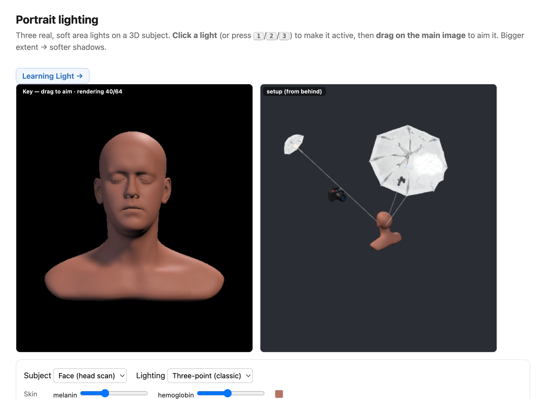
Bounce and off-camera. Never fire a bare flash straight at the subject — it gives flat, harsh light and red-eye. Bounce it off a ceiling or wall (~45°), or spread it with a diffuser, to enlarge the apparent light source and soften the shadows. Taking the flash off-camera entirely gives directional, shaped light (→ Computational illumination, including computational bounce flash, Davis et al. SIGGRAPH Asia 2016).

2.10.17 The traditional darkroom🔗⧉

A photograph is only half made when the shutter closes. For most of photography's history the other half happened in a darkroom, and it is worth knowing — both because film workflows are enjoying a revival and because nearly every tool in today's editing software is a darkroom operation in disguise.

The chemical pipeline has two stages. First the exposed film is developed: bathed in a developer that turns the exposed silver-halide grains to metallic silver, a stop bath that halts the reaction, and a fixer that dissolves away the unexposed grains so the image is no longer light-sensitive. The result is a negative — dark where the scene was bright. Then comes printing: an enlarger projects the negative onto a sheet of light-sensitive photographic paper, which is developed in its turn to give a positive print.

Printing is where the craft lives, because the enlarger is a second exposure that the printer fully controls:

• the exposure time under the enlarger sets the print's overall lightness — the global brightness knob;
• the contrast grade — the paper's grade, or a filter over the enlarger — sets how steeply scene tones map to print tones, the analog of a contrast or tone-curve control;
• dodging holds light back from a region (a hand or a paddle waved over it during the exposure) to make it lighter, while burning adds extra light to a region to make it darker — local tonal control, by hand.

This is the literal origin of the dodge and burn tools in Photoshop, of the exposure and contrast sliders everywhere, and of Ansel Adams's Zone System (the metering section's 18% gray is its Zone V) — a discipline for planning, at capture time, exactly where each scene tone will land on the print. The darkroom is also the concrete meaning of the book's recurring metaphor that the print is a performance of the negative (the score and the performance, and the measurement chapter's sidebar): two printers, one negative, two different photographs.

2.10.18 The digital darkroom: editing software🔗⧉

Today that darkroom is software, and it comes in two flavors worth telling apart, because they embody two different philosophies of editing (Figure 2.10.26).

Parametric raw "developers" — the Lightroom style. Adobe Lightroom, Capture One, Apple Photos, and the open-source darktable and RawTherapee are, at heart, raw developers wrapped in a library. They are non-destructive and parametric: the original file is never altered; every edit is stored as a small list of instructions applied on top of it, re-rendered live and reversible at any moment — the digital analog of deciding how to print a negative. The toolset is mostly global adjustments: white balance, exposure, contrast, highlights / shadows / whites / blacks, the tone curve, HSL (per-color hue/saturation/luminance), clarity / texture / dehaze, sharpening and noise reduction, lens corrections (distortion, vignetting, chromatic aberration), and crop / straighten — plus local adjustments painted in with masks, graduated and radial filters, and increasingly AI-driven subject and sky masks. The other half of the job is asset management: importing, rating, keywording, and searching tens of thousands of photos. This is the everyday workflow for most photographers, applied across whole shoots at once.

Pixel editors — the Photoshop style. Adobe Photoshop (and GIMP, Affinity Photo) work the other way: they manipulate the pixels directly, with layers, selections, and masks for compositing, and a deep toolbox for retouching — the clone stamp and healing brush to remove blemishes and distractions, content-aware fill to erase objects, dodge / burn tools (there they are again), curves and levels as adjustment layers, filters, text, and montage. This is where you do pixel-level surgery, combine several frames into one, and composite — the things a parametric developer is not built for.

In practice most serious workflows use both: develop and cull in a Lightroom-style tool, then hand the few keepers to Photoshop for heavy retouching or compositing. The dividing line is global, reversible, many-photos versus local, pixel-level, one-photo.

And here is the bridge into the rest of this book: every one of those tools is an algorithm, and we are going to study how each one works. The exposure and contrast sliders are point operations and tone curves (BASIC → Point operations, Tone mapping); the histogram you push for ETTR gets its own chapter (Histograms); white balance is color constancy (Color technology); sharpening, blur, and clarity are convolution and edge-preserving filtering (Neighborhood operations; Bilateral filtering); noise reduction is denoising; raw development is demosaicking; crop and straighten are resampling; content-aware fill and seamless compositing are Poisson editing and seam optimization (EDGES MATTER); and the newest "generative fill" and AI masking are diffusion models and learned segmentation (COMPUTATIONAL TOOLS). The slider is the interface; the rest of the book is the machinery underneath it.

This chapter has walked photography end to end — exposure, modes, focus, lenses and their filters, keeping the glass clean, stabilization, the viewfinder, video, programmability, the two anatomies that book-end the field (a full-frame body where good optics do the work, and a phone where computation does), the wider taxonomy of camera types and the many cameras that measure rather than photograph, and finally the post-capture darkroom, chemical and then digital. That last step is the hinge into the rest of the book: the phone is the machine the book is really about, and editing software is where its output is finished — and everything from the develop slider to content-aware fill is an algorithm we are about to study. The next parts build the pipeline — image representation, the ISP, multi-frame fusion, and the editing operations themselves — that lets a fingernail-sized sensor punch far above its physics.