
fig-light-journey · FUNDAMENTALS part opener — the journey of light: source → scene (reflection) → lens → sensor / retina → visual system, each step labelled with its chapter ✅
fig-light-models · three models of light: wave (λ) vs ray vs particle/photon propagation, and what each is good for 🟨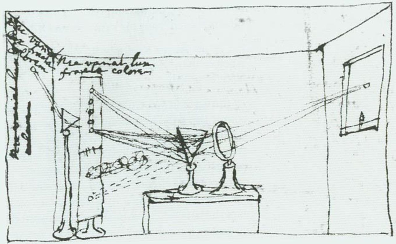
fig-newton-prism · Newton's prism experiment: white light dispersed into a spectrum (classic diagram) 🟨
fig-em-spectrum · EM spectrum / wavelength map 🟨
fig-reflection-refraction-diffraction · reflection (equal angles) · refraction (Snell, two indices) · diffraction 🟨
fig-polarization · unpolarized (random orientations) vs polarized light 🟨
fig-atmospheric-scattering · Rayleigh scattering: blue sky (short path) vs red sunset (long path) 🟨
fig-reflectance-illumination-spectra · example reflectance & illumination spectra 🟨
fig-illum-times-reflectance · light = illumination × reflectance (per-wavelength) ✅
fig-brdf · light bouncing off a surface — the BRDF (incoming/outgoing dirs, normal, reflection lobe, θ angles) 🟨
fig-diffuse-specular-spheres · Lambertian (matte) sphere vs shiny (specular) sphere — same shape/light, different BRDF 🟨
fig-global-illumination · color bleeding: a red wall casts red onto a white floor (multiple bounces) 🟨
fig-illuminant-spectra · blackbody / illuminant spectra (D65, tungsten, fluorescent) 🟨
fig-color-temperature · the (inverted) color-temperature scale: warm (low K) → cool (high K) 🟨
fig-radiance-irradiance · radiance (per direction) vs irradiance (per area) 🟨
fig-cosine-irradiance · why irradiance carries a cosine: a beam of width w vs its surface footprint L = w/cosθ 🟨
fig-seasons · sidebar — seasons: N. America in summer vs winter (sun angle → energy per area, cosine law) 🟨
fig-inverse-square-vs-radiance · point source 1/r² vs distance-invariant surface radiance 🟨
fig-diffraction-aperture-size · two apertures: a smaller one diffracts more (spread θ ≈ λ/D) 🟨
fig-airy-disk · Airy disk = diffraction-limited PSF 🟨
fig-aperture-sharpness-sweet-spot · aberration vs diffraction → sharpness sweet spot 🟨
fig-camera-obscura · camera obscura / pinhole (artist's) 🟨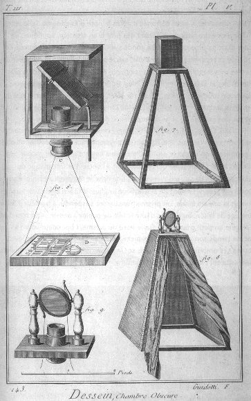
fig-camera-obscura-apparatus · camera obscura apparatus (Diderot engraving) 🟨
fig-bare-sensor-averaging · a bare sensor averages all rays 🟨
fig-pinhole-fov · pinhole geometry: real (inverted) vs virtual (upright) image plane, and focal length → field of view 🟨
fig-perspective-projection · perspective projection equation: x'=f·X/Z, y'=f·Y/Z (divide by depth, scale by f) 🟨
fig-perspective-projection-3d · perspective projection in 3D: P=(X,Y,Z) → p=(x,y) on the image plane through the pinhole 🟨
fig-perspective-vanishing-points · perspective projection + vanishing points 🟨fig-focal-length-compression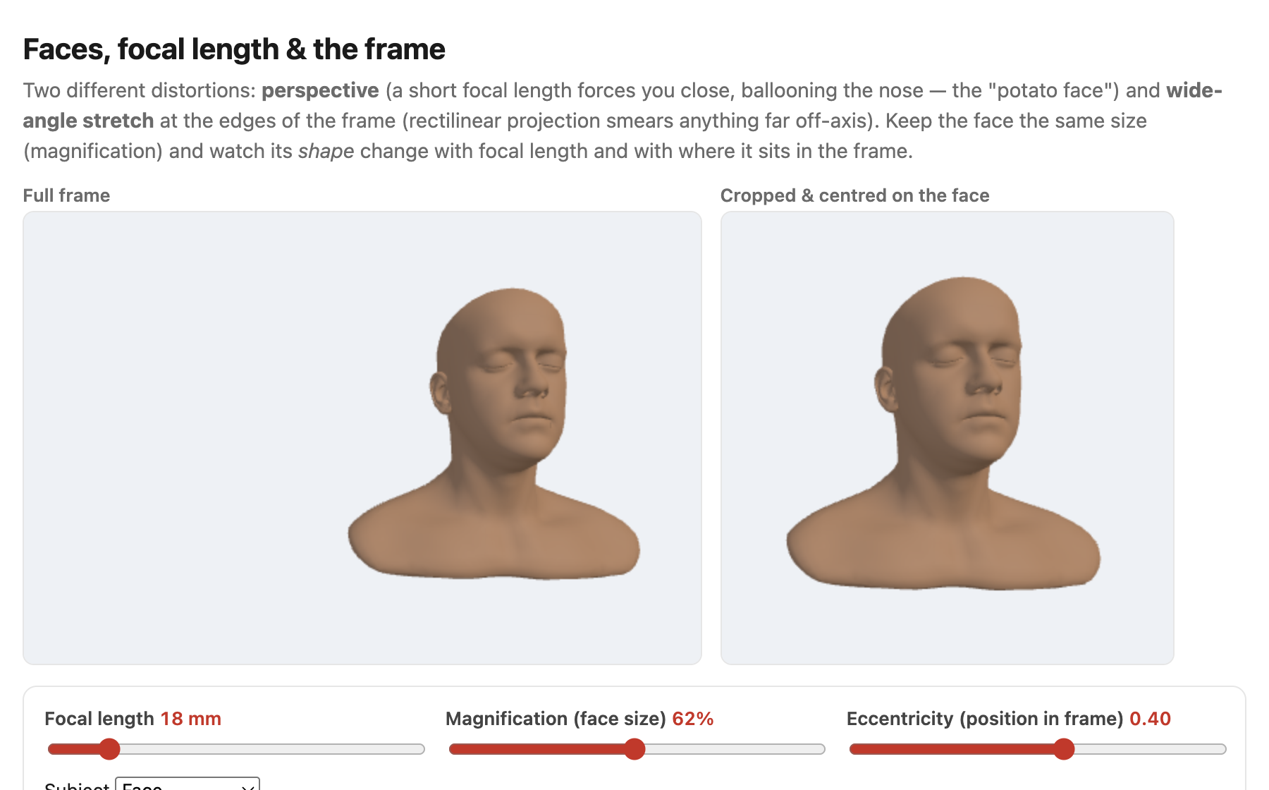
fig-face-distortion-sim · live face-distortion simulator (web edition): focal length + magnification + eccentricity controls with a full-frame view and a face-cropped view, showing the close-wide "big nose" perspective and the wide-angle edge stretch at constant face size; subject = a face, a grid sphere, or one of six diverse Meshy humans framed on the face; static fallback is a screenshot. *Human 3D models generated with Meshy AI.* ✅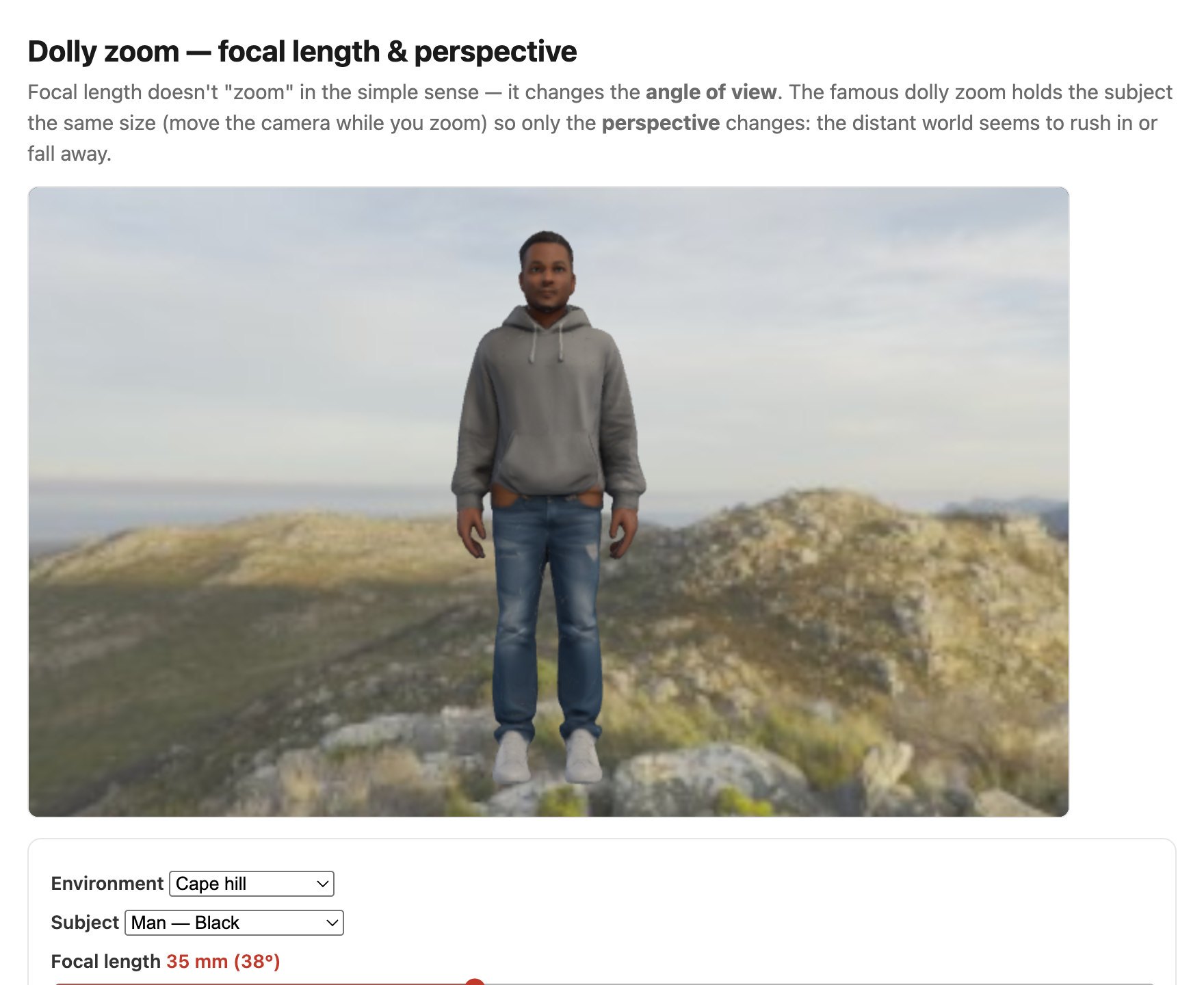
fig-dolly-zoom-sim · live dolly-zoom simulator (web edition): hold the subject size while focal length and camera distance trade off so only perspective / background scale changes; log focal (12–200 mm) + distance sliders, realistic Poly Haven environments, subject = head bust or one of six diverse Meshy humans. *Human 3D models generated with Meshy AI.* ✅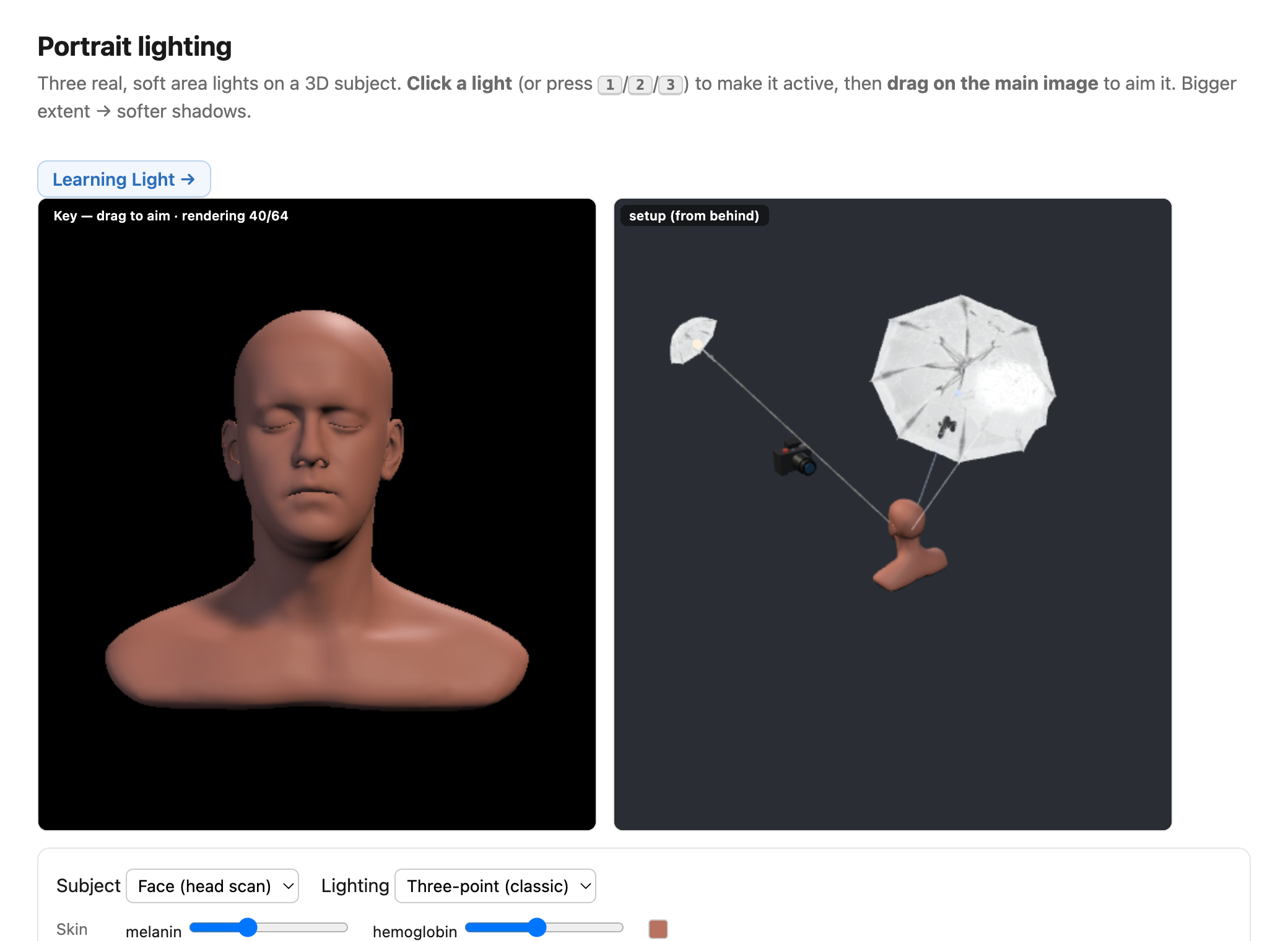
fig-portrait-lighting-sim · live portrait-lighting simulator (web edition): three soft area lights (key/fill/kicker — az/el/extent/intensity/colour, area-light-supersampled soft shadows) on a 3D face with a physiological melanin/hemoglobin skin model; a from-behind setup view with Meshy studio umbrellas + a camera rig; lighting presets; static fallback is a screenshot. *3D umbrella generated with Meshy AI.* ✅
fig-keystoning-cause · keystoning is the tilt, not the lens — a camera tilted up makes world-parallel verticals converge (façade → trapezoid), while the fronto-parallel shot keeps them parallel; projection preserves lines, not parallelism 🟨
fig-point-line-duality · point↔line duality in homogeneous 2D: two points → a line, two lines → a point (same cross product) 🟨
fig-projection-decomposition · projection-matrix decomposition K·[R matplotlib, 3-stage pipeline
fig-crop-focal-length · cropping = changing focal length: full frame vs a crop box ≡ a longer-focal-length capture, upsampled 🟨
fig-depth-vs-ray-length · depth (z coordinate) vs ray length ‖P‖ from camera to a 3D point; unproject (pixel + depth → 3D) 🟨
fig-single-lens-refraction · single lens, two interfaces, Snell at each → focus 🟨
fig-thick-lens-snell · thick lens: Snell's law at both interfaces, with the incidence/refraction angles and indices of refraction shown 🟨
fig-fermat-equal-path · the Fermat / equal-optical-path view of a lens: several rays object→focus, all the same optical path (glass detour offsets the slower speed) 🟨
fig-thick-lens-wave-sim · live 2-D FDTD wave sim of a **thick biconvex lens** focusing: a point source's diverging wave is reshaped by the slower glass into a converging one that meets at an image point; focus tracks 1/f=(n−1)2/R and 1/v=1/f−1/u (Fundamentals → Lens image formation, Fermat/equal-path) ✅
fig-thin-lens-rays · thin-lens ray diagram (focus, focal point) 🟨
fig-thin-lens-conjugates · conjugates: object at ∞ / far / close / at focal length → where the image forms 🟨
fig-circle-of-confusion · finite aperture & circle of confusion ✅
fig-defocus-vs-parameters · defocus blur (CoC) vs aperture and object distance 🟨
fig-depth-of-field · near/far limits where blur reaches c (linearized DoF) 🟨
fig-dof-derivation-near · near (front) limit by similar triangles — all quantities 🟨
fig-dof-derivation-far · far (back) limit by similar triangles — all quantities 🟨
fig-dof-vs-parameters · DoF vs aperture, focal length, focus distance 🟨
fig-hyperfocal · hyperfocal: focus at H → sharp from H/2 to ∞ 🟨
fig-dof-same-framing · same framing + same f-number → same object-space DoF (short vs long focal length); background blur still looks larger with the long lens 🟨
fig-dof-double-cone · object-space DoF as a double cone in front of the lens, waist on the focus plane (the blur for one scene point) 🟨
fig-dof-depth-dependent · defocus is NOT a convolution: blur radius depends on scene depth (not pixel location), and occlusion at depth edges 🟨
fig-dof-background-blur · DoF focal-length invariance is only first-order: background blur c vs background distance for 35/85/200 mm (matched framing & N) coincide near the subject and fan apart far away; + c vs focal length showing growth/saturation ✅
fig-contrast-af-curve · contrast-detect AF: high-frequency contrast (sharpness) vs focus position, peaked at best focus; hill-climb arrows that must overshoot past the peak then step back (no direction cue) ✅
fig-pixel-measurement-integral · a pixel value = integral over aperture (thin lens ellipse) + finite pixel area (+ time, wavelength); the 4 domains → DoF, antialiasing, motion blur, color; linked to the plenoptic function 🟨
fig-sensor-microlens · sensor cross-section: microlens → filter → photosite 🟨
fig-rolling-shutter-pan · a slanted, sheared vertical pole from an uncorrected fast pan vs a straightened, rectified version, illustrating line-by-line CMOS readout during camera motion 🟨
fig-slowmo-axis · four ways to treat the time axis on a shared timeline — normal capture (sparse), high-speed (dense true samples), interpolation (sparse reals with synthesized in-betweens), and long-exposure blur (the integral); only interpolation adds resolution after capture and can be wrong 🟨
fig-mirrorless-anatomy · labeled cutaway of a mirrorless full-frame camera (lens+mount, sensor/IBIS, mech+electronic shutter, EVF, processor/on-sensor PDAF, card+battery); SLR mirror-box inset for contrast ✅
fig-rolling-shutter-skew · rolling-shutter distortion — a global shutter keeping a vertical pole upright under a fast pan vs a rolling shutter where per-row readout $t(r)=t_\text{frame}+r\,t_\text{row}$ shears the pole and smears fan blades (the jello effect) 🟨
fig-flash-sync · flash & focal-plane-shutter sync: whole frame ≤ X-sync · slit/partial frame above it · high-speed-sync pulse train; fill-flash noted ✅
fig-darkroom-dodge-burn · the darkroom ancestor: dodging (hold back light) and burning (add light) under the enlarger as hand-painted spatially-varying exposure 🟨fig-noise-histogramfig-noise-vs-iso
fig-noise-affine · measured noise variance is affine in brightness (σ²≈gain·I+read²) — real per-pixel variance vs mean from a 50-frame aligned ISO-3200 burst, with the affine fit, read-noise floor, and highlight roll-off (Noise, SNR, dynamic range) ✅
fig-noise-gaussian-pixels · a single pixel's value across many frames is ≈ Gaussian — per-pixel histograms from the ISO-3200 burst with Gaussian overlays (Noise) ✅
fig-noise-truncation · noise clips at black/white so it is not zero-mean at the extremes — a near-black pixel pinned at 0 ~44% of frames, its average biased bright, vs an unbiased midtone (Noise; denoising trap) ✅
fig-snr-vs-stddev · noise std-dev map vs SNR map of a brightness ramp: std rises with brightness (∝√N), but SNR=√N is worst in the shadows 🟨fig-underexposure-recovery-ff-vs-phonefig-results-montage
fig-dynamic-range-comparison · dynamic-range ladder in **stops** (horizontal bars): colour slide (~5–6) · reflective print (~6–7) · film negative (~12–13) · phone sensor (~10–12) · full-frame sensor (~14) · human eye instantaneous (~10–14) vs adapted (~20+) · an animal example · a typical sun-and-shadow scene (>20) — shows why no single capture holds a high-contrast scene (→ HDR) ✅fig-stereo-pair
fig-disparity-geometry · parallel-camera disparity geometry 🟨fig-disparity-map
fig-random-dot-stereogram · a random-dot stereogram pair (Julesz): a shifted central patch → depth from disparity alone, no monocular cues 🟨
fig-epipolar-line · the epipolar constraint: two views of a 3-D point, epipolar plane & line, the match constrained to a 1-D search ✅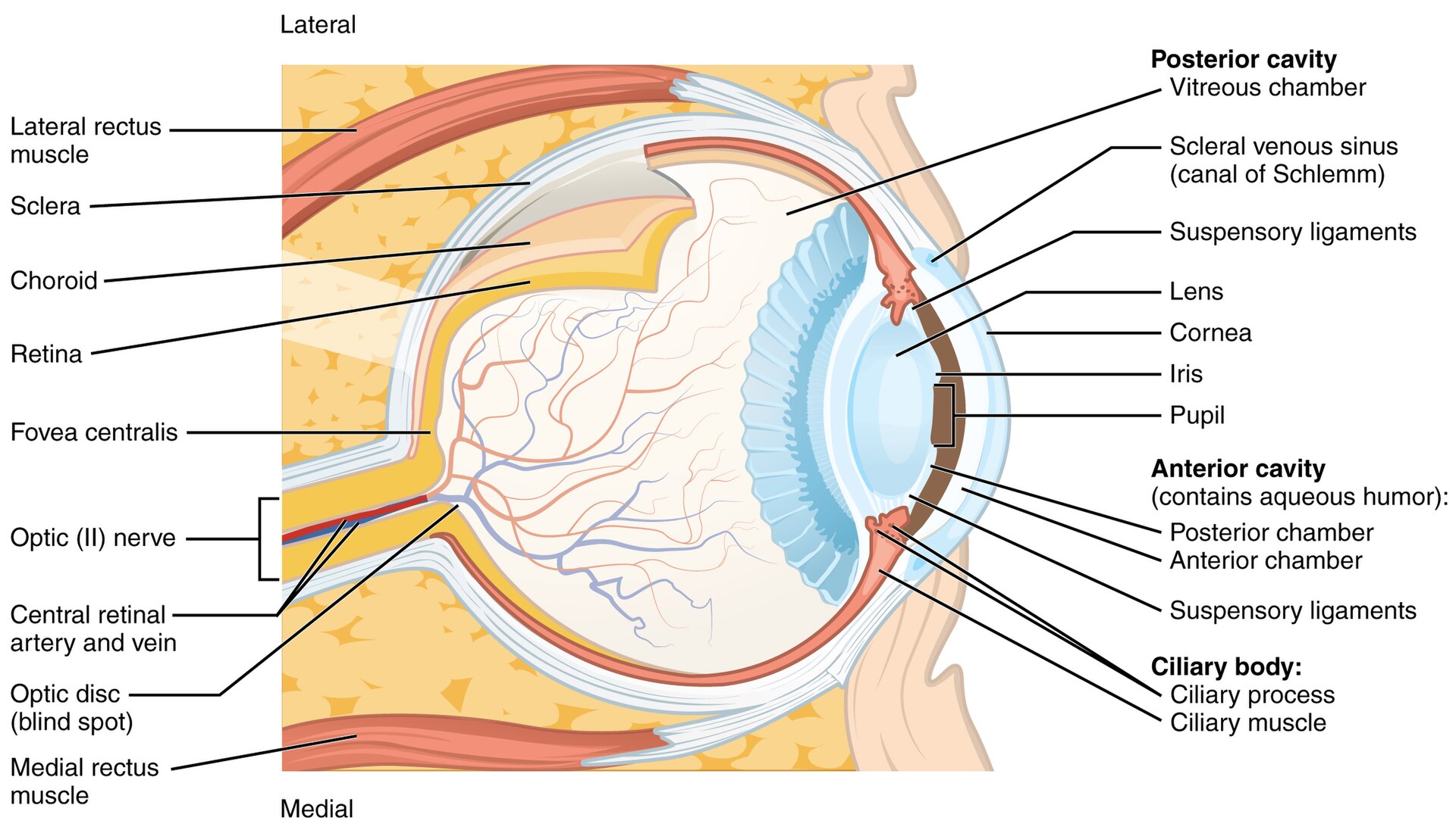
fig-eye-cross-section · eye cross-section 🟨
fig-retina-layers · retina layers & photoreceptor synapses 🟨
fig-cone-rod-distribution · cone/rod distribution & fovea 🟨
fig-visual-pathway · pathway retina→LGN→V1 🟨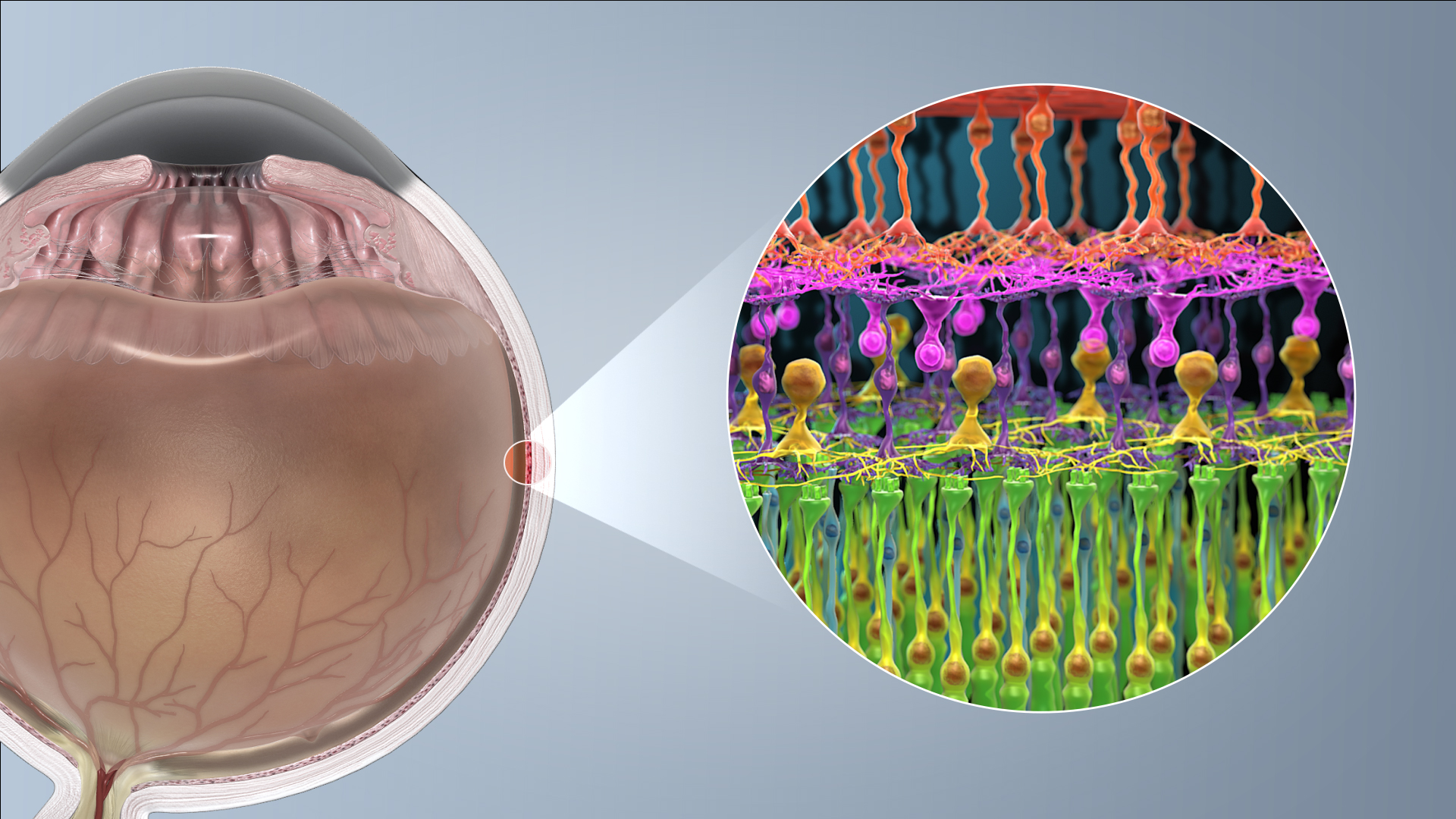
fig-photoreceptor-cell · anatomy of a rod & cone cell 🟨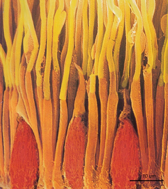
fig-rods-cones-micrograph · micrograph of rods & cones (primate retina) 🟨
fig-cone-sensitivities · cone spectral sensitivities (L/M/S) 🟨
fig-spectrum-to-three-responses · spectrum → 3 responses (projection) 🟨
fig-metamers · metamers (two spectra, one color) 🟨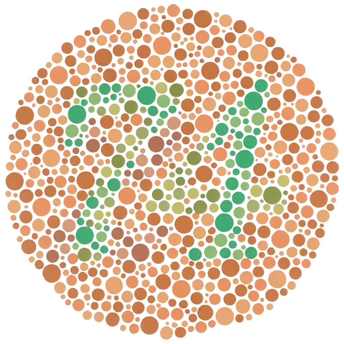
fig-ishihara · Ishihara plate (“74”) 🟨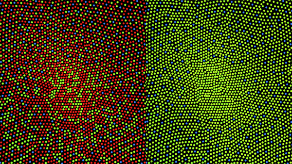
fig-cone-mosaic · trichromatic cone mosaic (L/M/S, fovea) 🟨
fig-cone-response-matrix · cone response as a 3×N matrix–vector product r = C·E (discretized λ); note the continuous / infinite-D limit r_k = ∫ c_k(λ) E(λ) dλ 🟨
fig-nonorthogonal-dual-basis · non-orthogonal cone basis (two vectors in the positive quadrant) and its dual: synthesis vs analysis; the dual (analysis) basis has negative coordinates 🟨
fig-opsin-tree · the opsin gene tree (schematic): ancestral opsin → RH1 rod + cone classes (SWS1/SWS2/RH2/LWS); the human S/M/L branch highlighted, with the recent primate L/M gene duplication marked ✅
fig-opponent-channels · opponent channels (R–G, B–Y, light–dark) 🟨
fig-afterimage · afterimage demo 🟨
fig-spanish-castle · afterimage / Spanish-Castle illusion ✅
fig-photopic-scotopic-range · the photopic / mesopic / scotopic regimes on a horizontal log-luminance axis (cd/m², ~10⁻⁶→10⁸): rod vs cone activity bands, the absolute threshold, the Purkinje shift, and landmarks (starlight, moonlight, indoor, overcast, sunlight, the sun); the eye's full range vs the few-log instantaneous range (→ adaptation, HDR) ✅
fig-checker-shadow · Adelson's checker-shadow illusion — the original artwork: the illusion (squares A/B identical luminance) beside the equal-grey-bars proof ✅
fig-white-balance-real · white balance computed from scratch (von Kries per-channel gain in linear light): a warm-casted photo corrected by gray-world vs white-patch/max-RGB, with the recovered channel gains (PS1) ✅fig-wb-before-afterfig-the-dress
fig-simultaneous-contrast · simultaneous-contrast patch 🟨
fig-mach-bands · Mach bands 🟨
fig-contrast-ratios · contrast-as-ratios strip 🟨
fig-campbell-robson · Campbell–Robson CSF chart 🟨
fig-acuity-chart · an acuity chart 🟨
fig-csf-chromatic · three contrast-sensitivity functions: luminance (band-pass) vs red–green and blue–yellow (low-pass, lower cutoff) — we resolve colour more coarsely than brightness 🟨
fig-blur-chroma-luma · blur only the chroma (Lab) and the image still looks sharp; blur the luminance and it falls apart — the basis for chroma subsampling ✅fig-scanpath
fig-hunt-effect · colorfulness vs luminance (Hunt) 🟨
fig-bezold-brucke-abney · Bezold–Brücke / Abney demos ✅
fig-eye-evolution · the evolution of the eye, in cross-sections: flat photoreceptor patch (no image) → cup (directional) → pinhole (an image, no lens) → lensed eye — recapitulating sensor → camera-obscura → lens (Bonus: animal eyes) 🟨
fig-analysis-vs-synthesis · analysis vs synthesis (sense→3 / reproduce←few) 🟨
fig-color-matching-setup · color-matching experiment setup ✅
fig-cie-cmfs · CIE color-matching functions 🟨
fig-chromaticity-diagram · xy chromaticity + spectral locus + white point 🟨
fig-gamma-curves · gamma encode/decode curves 🟨
fig-quantization-banding · quantization banding (low-bit demo), worst in shadows ✅
fig-slr-cross-section · labelled cross-section of an SLR: 45° main reflex mirror sends light UP to the focusing screen + pentaprism → optical viewfinder; the semi-transparent main mirror + secondary (sub) mirror fold light DOWN to the phase-detect AF module in the mirror-box floor; focal-plane shutter + sensor/film behind; inset shows the mirror flipping up for exposure (companion to `fig-mirrorless-anatomy`) ✅
fig-rgb-cube · RGB cube 🟨
fig-gamut-primaries · sRGB vs wide-gamut primaries on xy 🟨
fig-perceptual-uniformity · a rainbow at N colours equally spaced in sRGB vs CIELAB; ΔE bars under each strip show sRGB steps are perceptually ragged, CIELAB steps even (Color technology — CIELAB) 🟩
fig-cielab-space · CIELAB space 🟨
fig-cielab-ab-plane · the a*b* plane 🟨
fig-additive-subtractive · additive vs subtractive synthesis 🟨
fig-color-synthesis-bands · additive vs subtractive synthesis, 3-band cartoon; subtractive is multiplicative (Color technology) 🟨
fig-subtractive-spectra · subtractive mixing as a per-wavelength multiplication: yellow & cyan filter transmittances and their product T_Y·T_C (= green) 🟨
fig-gamut-mapping · gamut + gamut mapping 🟨
fig-repro-monochromatic · reproducing a monochromatic signal (2D LA analogy) 🟨
fig-icc-workflow · ICC workflow diagram 🟨
fig-device-gamut-mismatch · gamut mismatch across devices ✅
fig-color-multiplexing · four colour-sensing multiplexing strategies: temporal, spatial (Bayer), beam-split prism, depth (Foveon) 🟨fig-prokudin-gorskii
fig-point-op-saturation-vibrance · uniform saturation (constant `s`, over-saturates already-vivid colours → clip) vs vibrance (per-pixel gain `g = 1+v(1−sat)·w_skin(hue)`, protects vivid colours & skin): input, saturation, vibrance + a gain-vs-saturation panel (Point operations → Basic colour enhancement, BASIC) 🟩
fig-bw-conversions · one colour photo → black & white several ways: single channel (R/G/B) · average · weighted luminance · red-filter channel mix (dark sky) · an isoluminant pair collapsing to one grey — the choices differ (Converting to B&W, Color technology) ✅
fig-color-dimensions · the dimensions of color (hue/chroma/lightness) 🟨
fig-color-solid · a perceptual color solid ✅
fig-skin-tone-vectorscope · skin-tone locus on a vectorscope ✅fig-diverse-skin-tonesfig-shirley-card
fig-exposure-triangle · exposure triangle 🟨
fig-fstop-progression · f-stop power-of-two progression 🟨 pilot renderedfig-aperture-doffig-shutter-motion-blurfig-metering-18-gray
fig-ettr-histogram · expose-to-the-right: an image histogram pushed toward the highlights without clipping (vs an under-exposed one bunched at the noise floor) 🟨
fig-mode-dial · exposure mode dial (P/A/S/M) → who sets aperture vs shutter in the exposure triangle ✅
fig-telephoto-vs-retrofocus · two two-group schematics — telephoto (+ then −, principal plane H′ pushed in front → physical length < f) vs retrofocus/inverted-telephoto (− then +, long back-focal distance to clear the SLR mirror); marks f vs physical length, H′, F′ ✅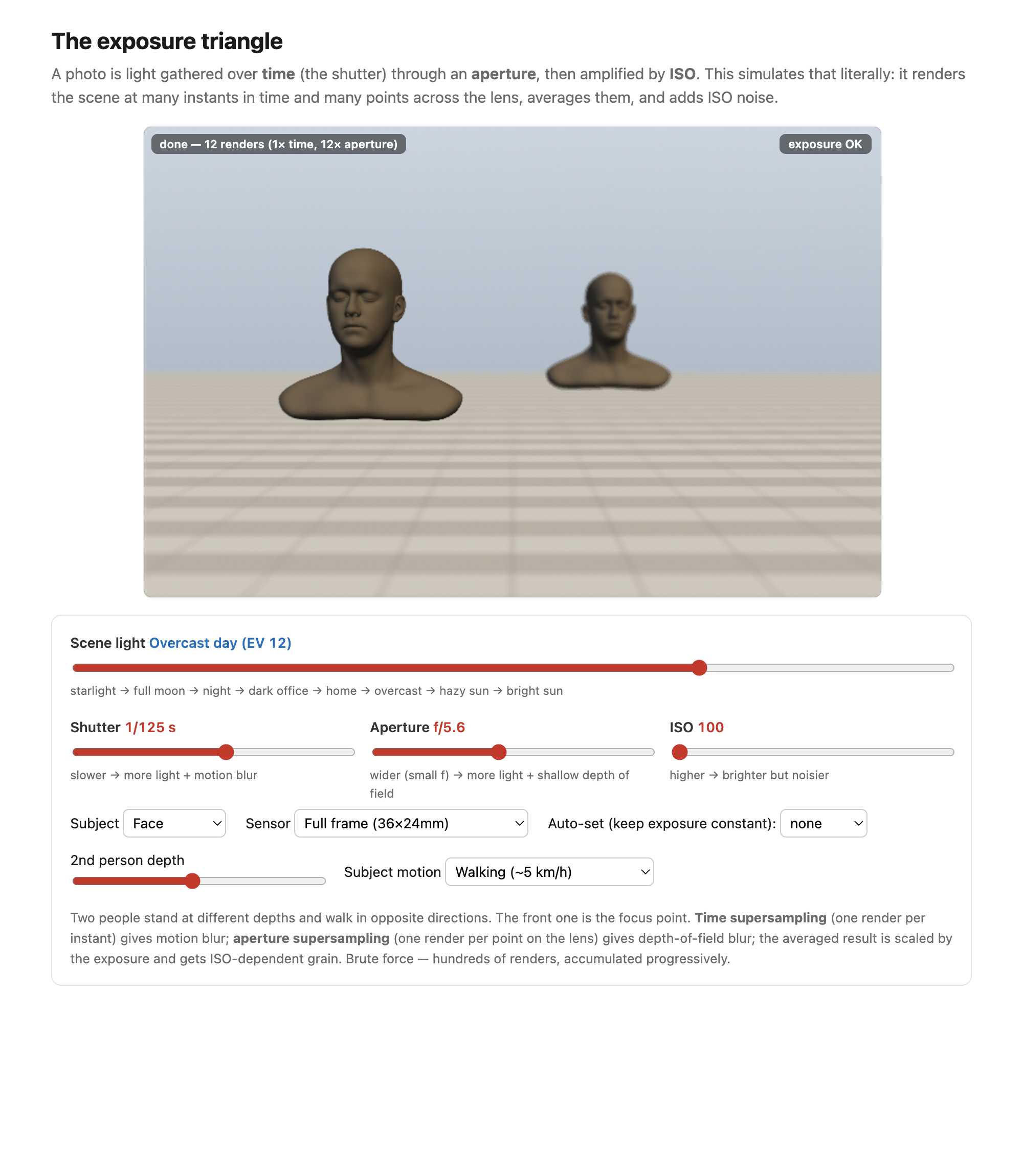
fig-exposure-triangle-sim · live exposure-triangle simulator (web edition): two 3D subjects at different depths walking opposite ways; shutter/aperture/ISO/scene-light/sensor sliders with brute-force time + aperture supersampling (real motion blur, depth of field, shot+read noise) and an auto-set triangle; static fallback is a screenshot ✅
fig-af-families · autofocus families: contrast-detect hill-climb · phase-detect sub-aperture offset · on-sensor/dual-pixel PDAF ✅fig-telephoto-vs-retrofocus · two two-group schematics — telephoto (+ then −, principal plane H′ pushed in front → physical length < f) vs retrofocus/inverted-telephoto (− then +, long back-focal distance to clear the SLR mirror); marks f vs physical length, H′, F′ ✅
fig-focus-conjugate-move · focusing geometry: as subject distance u changes the image distance v must change (1/f=1/u+1/v); the lens slides to keep the image plane on the fixed sensor — near vs far focus (lens extends vs retracts) ✅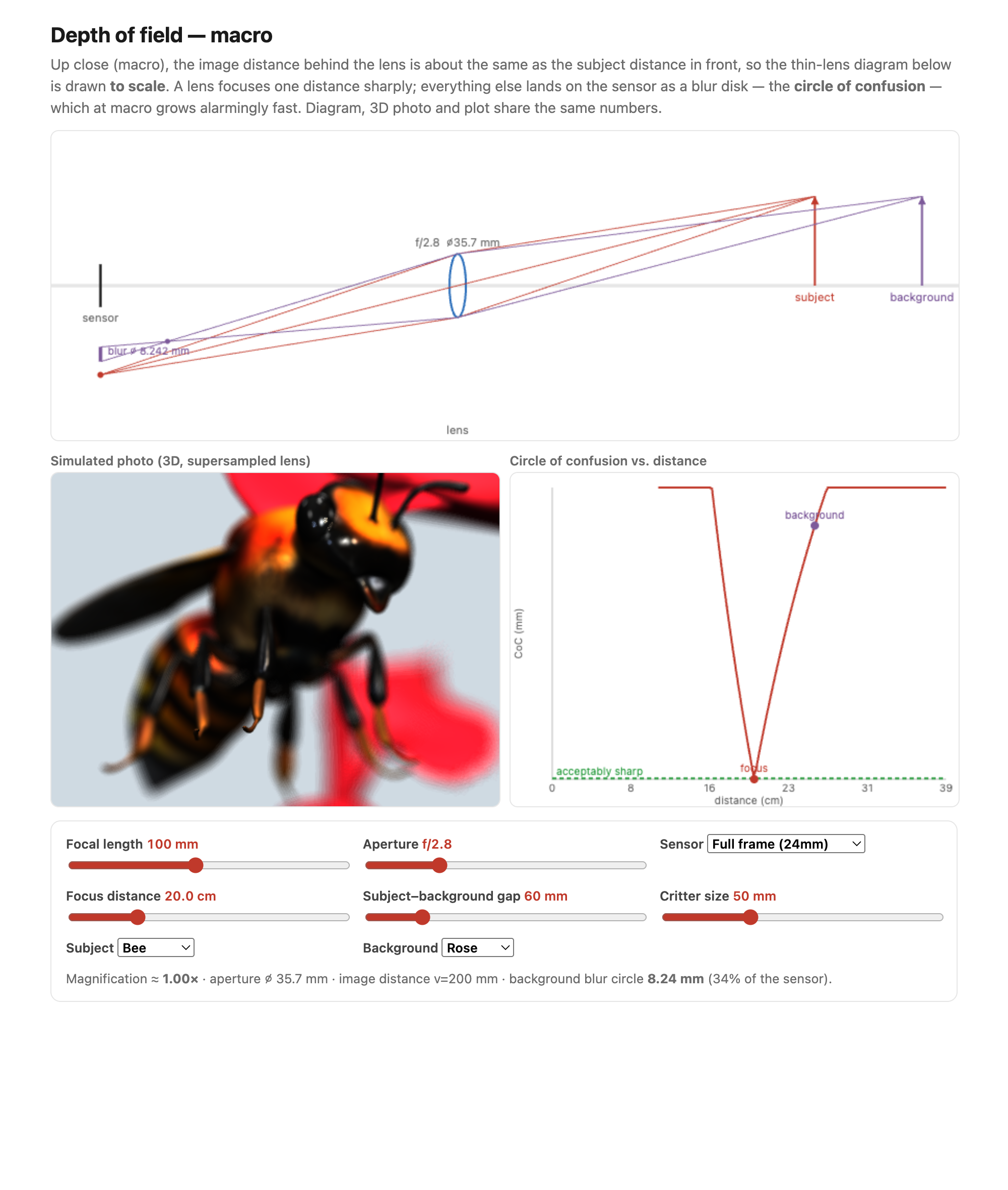
fig-depth-of-field-sim · live macro depth-of-field simulator (web edition): a to-scale thin-lens diagram + a 3D photo (aperture-supersampled bokeh) + a circle-of-confusion plot all sharing one optics model; subject dropdown (Meshy beetle / bee / ladybug) over a flower background, focus landing on the front of the face so the body and antennae blur; static fallback is a screenshot. *Bug & flower 3D models generated with Meshy AI.* ✅
fig-focal-length-families · focal-length families as nested FOV cones (ultrawide/wide/normal/short-tele/tele) with angle of view + one-word use each ✅fig-telephoto-vs-retrofocus · two two-group schematics — telephoto (+ then −, principal plane H′ pushed in front → physical length < f) vs retrofocus/inverted-telephoto (− then +, long back-focal distance to clear the SLR mirror); marks f vs physical length, H′, F′ ✅fig-dolly-zoom-sim · live dolly-zoom simulator (web edition): hold the subject size while focal length and camera distance trade off so only perspective / background scale changes; log focal (12–200 mm) + distance sliders, realistic Poly Haven environments, subject = head bust or one of six diverse Meshy humans. *Human 3D models generated with Meshy AI.* ✅
fig-reflection-removal-cues · cues that separate a window reflection from the transmitted scene — ghosting/double-image, polarization, focus difference 🟨fig-gain-vignette-solve
fig-jpeg-artifacts-photo · JPEG blocking & ringing on a REAL photographic edge (white egret vs dark foliage) at q=10: grid-aligned zoom with 8×8 overlay — blocking in the smooth area, ringing along the edge (File formats, BASIC) ✅
fig-lens-flare-ghosting · stray light: a bright source, a ray reflecting off two internal lens surfaces → a "ghost" landing displaced on the sensor, plus a veiling-glare wash; ghost vs flare labelled ✅
fig-ois-vs-ibis · two stabilization strategies side-by-side: lens-shift OIS (floating lens group moves) vs sensor-shift IBIS (sensor moves on a magnetic stage), moving element highlighted, same gyro/IMU input ✅fig-telephoto-vs-retrofocus · two two-group schematics — telephoto (+ then −, principal plane H′ pushed in front → physical length < f) vs retrofocus/inverted-telephoto (− then +, long back-focal distance to clear the SLR mirror); marks f vs physical length, H′, F′ ✅
fig-stabilization · image stabilization: hand-held blur vs OIS (lens shift) vs IBIS (sensor shift); ~2–5 stops, camera shake not subject motion ✅
fig-viewfinder-types · viewfinder types: OVF (optical) vs EVF (electronic) vs rear LCD ✅fig-telephoto-vs-retrofocus · two two-group schematics — telephoto (+ then −, principal plane H′ pushed in front → physical length < f) vs retrofocus/inverted-telephoto (− then +, long back-focal distance to clear the SLR mirror); marks f vs physical length, H′, F′ ✅fig-ettr-histogram · expose-to-the-right: an image histogram pushed toward the highlights without clipping (vs an under-exposed one bunched at the noise floor) 🟨fig-depth-of-field-sim · live macro depth-of-field simulator (web edition): a to-scale thin-lens diagram + a 3D photo (aperture-supersampled bokeh) + a circle-of-confusion plot all sharing one optics model; subject dropdown (Meshy beetle / bee / ladybug) over a flower background, focus landing on the front of the face so the body and antennae blur; static fallback is a screenshot. *Bug & flower 3D models generated with Meshy AI.* ✅
fig-shutter-angle · shutter angle sets the blur — a rotating-disc shutter at $0°/180°/360°$ admitting a smaller/larger fraction of the frame interval $T$; $180°$ ($\tau=T/2$) is the cinematic film-look, small angles strobe 🟨fig-rolling-shutter-skew · rolling-shutter distortion — a global shutter keeping a vertical pole upright under a fast pan vs a rolling shutter where per-row readout $t(r)=t_\text{frame}+r\,t_\text{row}$ shears the pole and smears fan blades (the jello effect) 🟨
fig-bokeh-shapes · bokeh: out-of-focus highlights take the aperture's shape — circular (many blades / wide open) vs polygonal (few blades, stopped down); synthetic defocus-disk fields + aperture insets ✅fig-mirrorless-anatomy · labeled cutaway of a mirrorless full-frame camera (lens+mount, sensor/IBIS, mech+electronic shutter, EVF, processor/on-sensor PDAF, card+battery); SLR mirror-box inset for contrast ✅fig-telephoto-vs-retrofocus · two two-group schematics — telephoto (+ then −, principal plane H′ pushed in front → physical length < f) vs retrofocus/inverted-telephoto (− then +, long back-focal distance to clear the SLR mirror); marks f vs physical length, H′, F′ ✅
fig-phone-camera-array · phone multi-camera array (ultrawide/wide/tele+periscope, tiny sensors, bright fixed lenses) → a computational-pipeline block → final photo ✅fig-telephoto-vs-retrofocus · two two-group schematics — telephoto (+ then −, principal plane H′ pushed in front → physical length < f) vs retrofocus/inverted-telephoto (− then +, long back-focal distance to clear the SLR mirror); marks f vs physical length, H′, F′ ✅fig-newton-prism · Newton's prism experiment: white light dispersed into a spectrum (classic diagram) 🟨fig-dynamic-range-comparison · dynamic-range ladder in **stops** (horizontal bars): colour slide (~5–6) · reflective print (~6–7) · film negative (~12–13) · phone sensor (~10–12) · full-frame sensor (~14) · human eye instantaneous (~10–14) vs adapted (~20+) · an animal example · a typical sun-and-shadow scene (>20) — shows why no single capture holds a high-contrast scene (→ HDR) ✅
fig-lens-design-tradeoff · lens-design Pareto cartoon as a 6-axis radar (sharpness, speed, size, weight, cost, distortion): fast pro prime vs compact phone lens overlaid, plus a dashed polygon showing where software correction shifts the phone lens (Lens optimization) ✅
fig-lagrangian-vs-eulerian · the organizing diagram — Lagrangian (arrows following particles over time → flow and tracking, output trajectories) vs Eulerian (a fixed grid, each pixel plotting intensity-over-time → magnification, never asking where anything went) 🟨
fig-pinhole-imaging · imaging-scenario series (2/3): add a pinhole to the bare sensor — one ray per scene point → a dim **inverted** image (same tree+sensor+colours as fig-bare-sensor-averaging) ✅fig-telephoto-vs-retrofocus · two two-group schematics — telephoto (+ then −, principal plane H′ pushed in front → physical length < f) vs retrofocus/inverted-telephoto (− then +, long back-focal distance to clear the SLR mirror); marks f vs physical length, H′, F′ ✅
fig-point-op-levels · levels on a real (flat/hazy) photo: bunched-up luma histogram stretched out to fill [0,1] by setting a black point and a white point — input + after + transfer curve with the clip-and-stretch anchors and the two histograms (Point operations → Black point, white point, and levels, BASIC) ✅
fig-wide-angle-perspective-distortion · wide-angle perspective distortion: off-axis spheres image as radially-stretched ellipses (flat-sensor geometry), and faces near a wide frame's edge are widened — not a lens flaw; forward-ref to correction (Pinhole image formation) ✅fig-flash-sync · flash & focal-plane-shutter sync: whole frame ≤ X-sync · slit/partial frame above it · high-speed-sync pulse train; fill-flash noted ✅fig-telephoto-vs-retrofocus · two two-group schematics — telephoto (+ then −, principal plane H′ pushed in front → physical length < f) vs retrofocus/inverted-telephoto (− then +, long back-focal distance to clear the SLR mirror); marks f vs physical length, H′, F′ ✅fig-darkroom-enlargerfig-telephoto-vs-retrofocus · two two-group schematics — telephoto (+ then −, principal plane H′ pushed in front → physical length < f) vs retrofocus/inverted-telephoto (− then +, long back-focal distance to clear the SLR mirror); marks f vs physical length, H′, F′ ✅fig-editing-lr-vs-ps